The heat capacity per unit horizontal area is : mass density times specific heat capacity times atmospheric depth. Thus is the rate of stored thermal energy per unit area. The solar constant is the incident radiative flux on a surface normal to sunlight; the ratio of the Earth's intercepting disk area to its spherical area is . The absorbed fraction is , where albedo is the reflected fraction. The outgoing radiative flux is , a Stefan–Boltzmann law with effective radiation factor incorporating the simplified greenhouse effect. Every term therefore has units of power per area.
The albedo curve decreases smoothly, passes through , and approaches at high temperature. At it is , close to when is large. Its derivative isAn ice-covered planet reflects more sunlight than exposed land or ocean. Warming removes reflective ice, lowers albedo, and increases absorbed radiative flux: this is ice-albedo feedback. The parameter controls the sharpness of this transition; the formula is an idealized global response, rather than a local melting law.
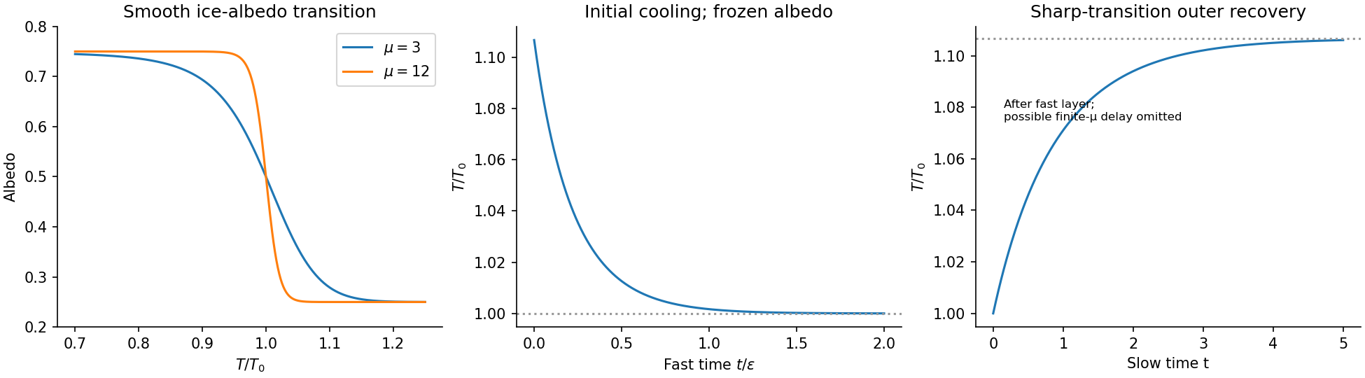
Temperature-dependent albedo and the separated fast cooling and slow recovery
. Details. Set . Since , the steady state energy balance is . Substitution givesThe two sides have slopes and at the origin. For , is strictly concave, its initial slope is , and it remains below . Consequently no positive root exists for , while for there is exactly one positive root . Oddness supplies the corresponding negative root. At the only root is still zero. Hence multiple steady temperatures occur precisely when .
The largest root corresponds monotonically to the largest positive absolute temperature:For large , the positive root tends to , so and . The negative branch has larger albedo and lower temperature.
Use dimensional quantities and set , . Dividing the energy balance by and the albedo equation by its time scale givesThus is the ratio of the atmospheric thermal response time to the much longer albedo response time. Converting kilometres to metres and years to seconds gives , , , andThe thermal time is about half a year, compared with a millennium for albedo adjustment. This is a singular perturbation: setting removes the independent initial condition for temperature.
Initially and , so . On the fast time , albedo changes by only andThus temperature rapidly falls towards . At the same time while , which seeds selection of the warm branch. Afterwards the approximate slow manifold is : decreasing albedo makes temperature rise slowly back towards . The preceding figure separates these two time scales; a single time axis would compress the initial fall into a nearly vertical segment.
In the sharp-transition regime, after selection of the warm branch . Solving the linear ordinary differential equation with the leading matched value givesThese are outer solutions: their initial temperature is , so the fast cooling layer is required to satisfy the actual initial temperature.
There is a useful qualification to the two-limit argument. For fixed finite , put on the slow manifold. Then , and is an unstable equilibrium with growth rate . The small positive seed from the fast layer can therefore produce a delay of order . The simple exponential approximation assumes that the sharp albedo transition is sufficiently fast to make this delay negligible on the displayed slow scale. It is not a uniform approximation for every fixed as .
Assume constant mass density, a prismatic channel, approximately uniform cross-sectional velocity , a hydrostatic pressure distribution, small bed slope , and no lateral inflow. Integrating mass conservation over a slice of length gives , hence .
Let be the hydrostatic first moment, where is the actual free-surface depth. The downstream momentum balance isUsing reduces its left side to . For a fixed prismatic cross-section, , so . Therefore the exact depth-averaged result isHere hydraulic radius converts perimeter shear stress into force per unit fluid volume. The printed notation yields the requested equation if it denotes this hydraulic pressure head, whose derivative equals .
The geometrical definition printed in the next part needs care. Triangular-channel hydrostatic pressure head gives the factor explicitly. For the stated symmetric triangular notch, the actual depth is , whereas its printed is . Indeed and , giving . Thus the equation with precisely the printed geometrical has pressure term . A first-principles derivation cannot remove that factor. The subsequent intended scaling can be carried out algebraically using the printed convention, as below, or with the pressure scale doubled for the actual triangular channel.
Write , , where the given geometry givesTake a Chézy drag law and restrict to downstream flow . Choose an area scale , length scale , and speed scale satisfyingThis makes gravitational driving and drag equal in the reference uniform steady flow. Dividing the printed momentum equation by givesMass conservation retains . In this notation is the square of the velocity-to-gravity-wave-speed ratio based on the chosen depth scale; authors sometimes instead denote its square root by Froude number. If the actual triangular pressure head from the preceding solution is used, replace by in both parameter definitions. The displayed dimensionless form remains the same, with consistently redefined parameters.
First neglect inertia relative to the pressure correction, requiring for smooth fields on these scales. The positive velocity isMultiplying by area gives the discharge . HenceThe leading equation is a nonlinear kinematic wave equation. The pressure correction has positive diffusion coefficient for and smooths steep gradients. Dropped terms are and inertial terms on the assumed scales; sufficiently thin fronts require a separate balance rather than an unrestricted Taylor expansion.
Let the original area be and the increased upstream area be . At , the conservation law flux is strictly convex. Characteristics behind the increase travel faster than those ahead, forming an admissible shock wave. Rankine-Hugoniot conditions give its speedAt the idealized hydrograph jumps from to at . With positive , the diffusion term spreads the rise over a finite interval. The hydrograph is rounded, with an earlier small response and a later approach to the new discharge, rather than an instantaneous jump.
The physical cause is the longitudinal pressure gradient: a local increase in depth influences neighbouring sections and redistributes water before pure downstream transport would deliver a discontinuity. For a small increase, linearization about has speed and diffusivity . The smooth curve in the figure is the exact half-line step response for this linearized advection-diffusion equation; it illustrates the shape without claiming to solve a large nonlinear jump exactly.
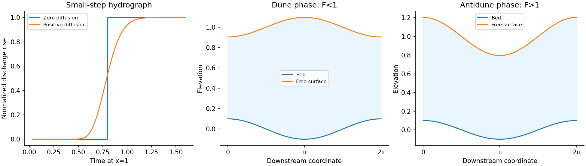
Sharp and diffused downstream hydrographs, with subcritical and supercritical bed-surface phases
. Details. The water mass conservation equation inherited from the earlier model is . It is essential: without it the printed displayed equations are not closed. Take the slow bed branch , and perturb the uniform state by , , , and . For , mass conservation gives and .
Put ; the extra comes from linearizing . The linearized momentum and suspended-sediment equations areEliminating gives the dispersion relationAway from , for fixed nonzero and negligible ,Thus growth requires . For , any gives an unstable branch; for growth would require . A physically increasing erosion function therefore gives the supercritical instability in this simplified model, rather than proving growth of ordinary subcritical dunes. Retaining drag giveswhich shows its stabilizing correction and the need to reconsider the limit near critical flow.
The negative bed-to-surface ratio for subcritical flow means bed crests lie beneath surface troughs: the dune phase relation. Its positive sign for supercritical flow gives aligned crests: an antidune. In the unstable supercritical case the imaginary part gives upstream migration, since . The figure shows these two phase relations. They identify the bedforms but do not by themselves establish growth. The qualitative limitation of the suspended-sediment mechanism is also discussed in the official [ref]
https://people.maths.ox.ac.uk/hewitt/publications/C5_11_notes.pdf. Mathematical Geoscience notes, pages 41–42
.Resolve gravity into components down the bed and normal to it. For slow incompressible flow, inertia is negligible and Cauchy momentum equation reduces to the divergence of the stress tensor plus the gravitational force density being zero. Write the dominant shear component as and the leading normal stresses as .
The shallow-ice approximation assumes a small thickness-to-length ratio. Vertical variation of the shear is retained in the along-bed equation, while longitudinal deviatoric-stress gradients and the shear contribution to the normal equation are higher order. The leading balances are consequentlyThe second is a hydrostatic pressure balance; the first balances gravitational driving and the surface-induced pressure gradient against vertical shear. This approximation requires shallow geometry and sufficiently slow flow, not a Newtonian constitutive equation for ice.
Measure pressure relative to atmospheric pressure. At leading order the stress-free upper surface gives , . Integrating the normal balance first yieldsAt fixed , . Therefore , independent of . Integrating from to givesThis is linear in , is zero at the surface, and reaches its basal value at . In particular the surface slope modifies the shear driving; a flat upper surface relative to the horizontal eliminates it in this approximation.
Set . For downstream shear , Glen's flow law and the no-slip boundary condition giveHere is the ice rate factor, distinct from the cross-sectional area in the river problem. Integrating this velocity profile through the thickness gives the volume flux per unit valley width:The factor combines the depth-dependent shear stress, integration to obtain velocity, and integration to obtain flux. If reverse shear is admitted for noninteger , the signed version of Glen's flow law is ; the displayed unsigned power presumes the downstream regime.
A typical net ice accumulation curve decreases downstream: snow gain at high elevation, zero at the equilibrium line, and negative values in the ice ablation zone. In a steady glacier with zero volume flux at its head, . If its terminus also has zero volume flux, a natural glacier length is the positive root of , with the integral positive between the endpoints. Such a root requires a suitable given accumulation profile; it is not guaranteed by dimensional analysis alone.
Let be a representative accumulation rate and . ChooseUsing , , , , , both terms in mass conservation have scale . The dimensionless flux isDropping hats gives the required partial differential equation. The parameter measures the surface-thickness slope correction relative to the bed slope. For the linear example , accumulation changes sign at and its integrated balance vanishes at .
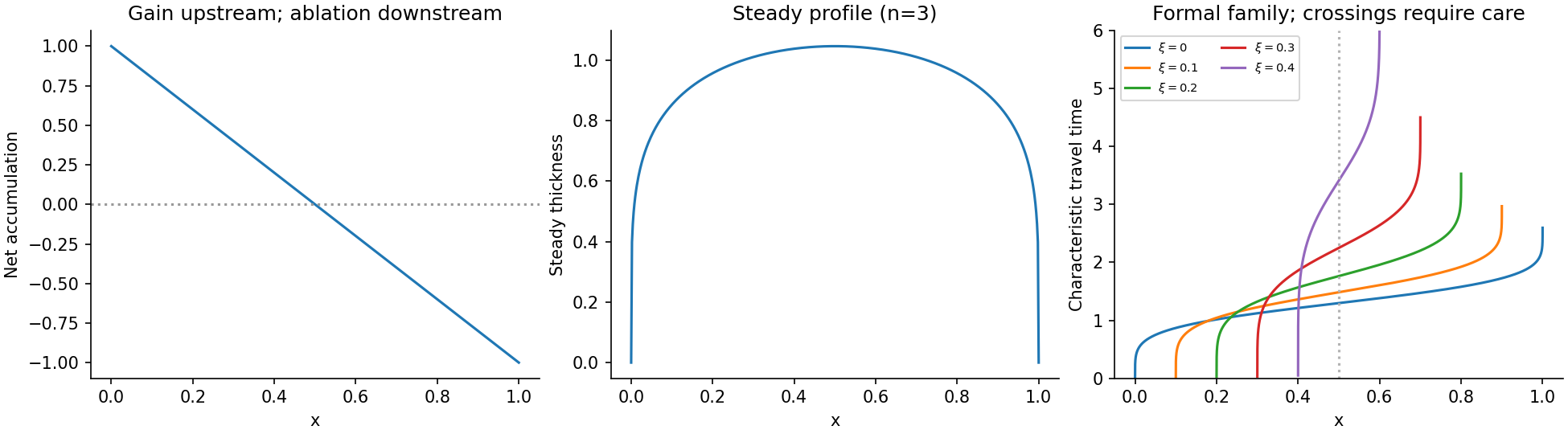


Write , and . Integrating the steady mass conservation equation from the head givesFor the time-dependent first-order equation , method of characteristics gives and . Consequently . On a characteristic starting at with zero thickness,On a characteristic emitted by the boundary , the invariant is zero and . The travel time of the one emitted at time zero isThe incomplete beta function is finite at both endpoints because for the physical exponents . Before characteristic crossings, the initial-data branch and boundary-data branch have the displayed forms in the source, with the appropriate emission time for the latter.
Glacier characteristic admissibility gives a substantive domain restriction. Factoring the invariant gives . A positive forward branch requiresEquivalently it is the image of this parameter domain under , restricted further to regions where that map is single-valued. Characteristics cannot start with positive thickness growth at , where the prescribed initial rate is negative. This is why the printed piecewise expression is a formal characteristic construction, not a global nonnegative solution from a bare bed. For example for , putting givesBoth factors increase with there, so no positive initial-data branch exists at that for , contrary to a literal global reading of the first case. Compression can also make characteristics intersect; entropy solutions then require shock waves.
One can nevertheless give the exact zero-thickness endpoint locus of these formal characteristics. Let . At the change of variable givesThis is the formal snout locus inferred from the given characteristic family; it retreats from towards . It is not justified as the physical terminus of an accumulating glacier formed from zero initial ice. In particular it says nothing about a positive advancing snout at . A physical free boundary problem must specify no ablation on a bare bed, maintain , and select an entropy solution or retain the small slope regularization. Those additional conditions are absent from the printed first-order construction. Thus a unique global physical snout trajectory cannot be claimed from that construction alone. The steady endpoint remains . The degenerate limit would instead have the same endpoint time for every initial characteristic, so the inverted formula presumes .
Articles by others on the same topic
There are currently no matching articles.