Principal component analysis replaces correlated measurements by orthogonal linear coordinates ordered by their variance. For centered observations collected in an matrix , write the sample covariance matrix as . A unit loading vector gives score vector with sample variance . The Rayleigh quotient is maximized by a unit eigenvector of for its largest eigenvalue.
The subsequent principal components maximize the same quadratic form subject to orthogonality to the earlier loading vectors. By the spectral theorem, if with descending eigenvalues, the scores have diagonal covariance . Their fractions of explained variance are . Repeated eigenvalues identify an eigenspace rather than a unique axis.
Keeping the first principal components gives the rank- reconstruction . Its squared reconstruction error isFor any rank- orthogonal projection , retained variance is . The weights lie in and sum to , so this is at most the sum of the largest eigenvalues. Projecting onto any candidate reconstruction subspace is its best least-squares reconstruction; this proves the minimum-error property and agrees with the singular value decomposition. Thus PCA finds the linear subspace preserving the greatest variance, equivalently minimizing squared reconstruction error. The upper-left sketch shows the first axis aligned with the elongated cloud; the second is perpendicular. A scree plot and substantive interpretability help choose .
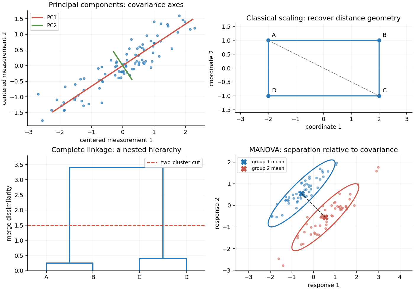
Original sketches of principal components, classical scaling, hierarchical clustering and multivariate mean comparison
. Details. 
These methods depend on measurement scale. A variable measured in large numerical units can dominate covariance-based principal component analysis; standardizing variables gives principal component analysis on a correlation matrix. Scores summarize patterns, but the method neither establishes causation nor guarantees that the largest-variance directions best predict a separate response.
Articles by others on the same topic
There are currently no matching articles.