Let each observation have dimension , and define the sample mean and the divisor- sample covariance matrix byThe multivariate normal distribution gives the log-likelihoodWriting makes the cross terms vanish, and the last sum becomes . Since is a positive-definite matrix, its minimum over the mean is at . ConsequentlyWhen is a positive-definite matrix, . Thuswhere depends on the data but not on .
For the maximum-likelihood estimator, consider the positive-definite matrix , with positive eigenvalues . The part of the profile likelihood depending on is . The elementary inequality , with equality exactly at , shows that the unique maximizing matrix is . HenceThe divisor is , not the unbiased covariance divisor . The regularity qualification matters: if is singular, the displayed logarithm of its determinant is not finite, and no positive-definite covariance maximizes the likelihood. Sending the fitted variance in a null direction of to zero makes the likelihood unbounded. For a nonsingular normal population, is positive definite almost surely when , which is the setting of the large-sample test.
Under the diagonal covariance restriction, the profile log-likelihood separates into terms,Differentiating each term gives the restricted maximum-likelihood estimator . Both fitted trace terms equal , so the likelihood-ratio test statistic iswhere is the sample correlation matrix. The statistic is nonnegative by the Hadamard inequality; large values indicate dependence. Equivalently, the likelihood ratio is and rejection is for small values of this ratio.
For fixed and a positive-definite true covariance, the Wilks theorem says that twice the maximized log-likelihood difference for nested regular models converges under the null to a chi-squared distribution with degrees of freedom equal to the dimension difference. The unrestricted covariance has parameters and the restricted covariance has ; the unknown mean has the same parameters in both. Therefore the Gaussian covariance diagonality likelihood-ratio test of asymptotic level isWithin the multivariate normal distribution, diagonal covariance also means independent coordinates.
Treat the displayed entries as the lower triangle of a symmetric sample covariance matrix , in the order mechanics, vectors, algebra, analysis, statistics. Compute the precision matrix . For a multivariate normal distribution, conditioning on all remaining coordinates givesThese identities follow by fixing the other coordinates in the quadratic form of the normal density and completing the square. For the second identity, the conditional precision matrix for the retained pair is its principal block; inverting that block gives the negative off-diagonal entry divided by the square root of the two diagonal entries.
Thus the two quantities to evaluate areAn equivalent procedure uses the Schur complement covariance: regress mechanics on the other four variables, or regress analysis and statistics separately on the remaining three. The first residual variance is ; the second result is the partial correlation of the two residuals. No arithmetic is required to specify this method.
The model qualification is important: a covariance matrix alone determines linear-regression residual variances and partial correlations. Identifying them with conditional quantities independent of the observed conditioning values uses the multivariate normal model, or another model with the same conditional moments; it does not follow for arbitrary distributions.
Principal component analysis replaces correlated measurements by orthogonal linear coordinates ordered by their variance. For centered observations collected in an matrix , write the sample covariance matrix as . A unit loading vector gives score vector with sample variance . The Rayleigh quotient is maximized by a unit eigenvector of for its largest eigenvalue.
The subsequent principal components maximize the same quadratic form subject to orthogonality to the earlier loading vectors. By the spectral theorem, if with descending eigenvalues, the scores have diagonal covariance . Their fractions of explained variance are . Repeated eigenvalues identify an eigenspace rather than a unique axis.
Keeping the first principal components gives the rank- reconstruction . Its squared reconstruction error isFor any rank- orthogonal projection , retained variance is . The weights lie in and sum to , so this is at most the sum of the largest eigenvalues. Projecting onto any candidate reconstruction subspace is its best least-squares reconstruction; this proves the minimum-error property and agrees with the singular value decomposition. Thus PCA finds the linear subspace preserving the greatest variance, equivalently minimizing squared reconstruction error. The upper-left sketch shows the first axis aligned with the elongated cloud; the second is perpendicular. A scree plot and substantive interpretability help choose .
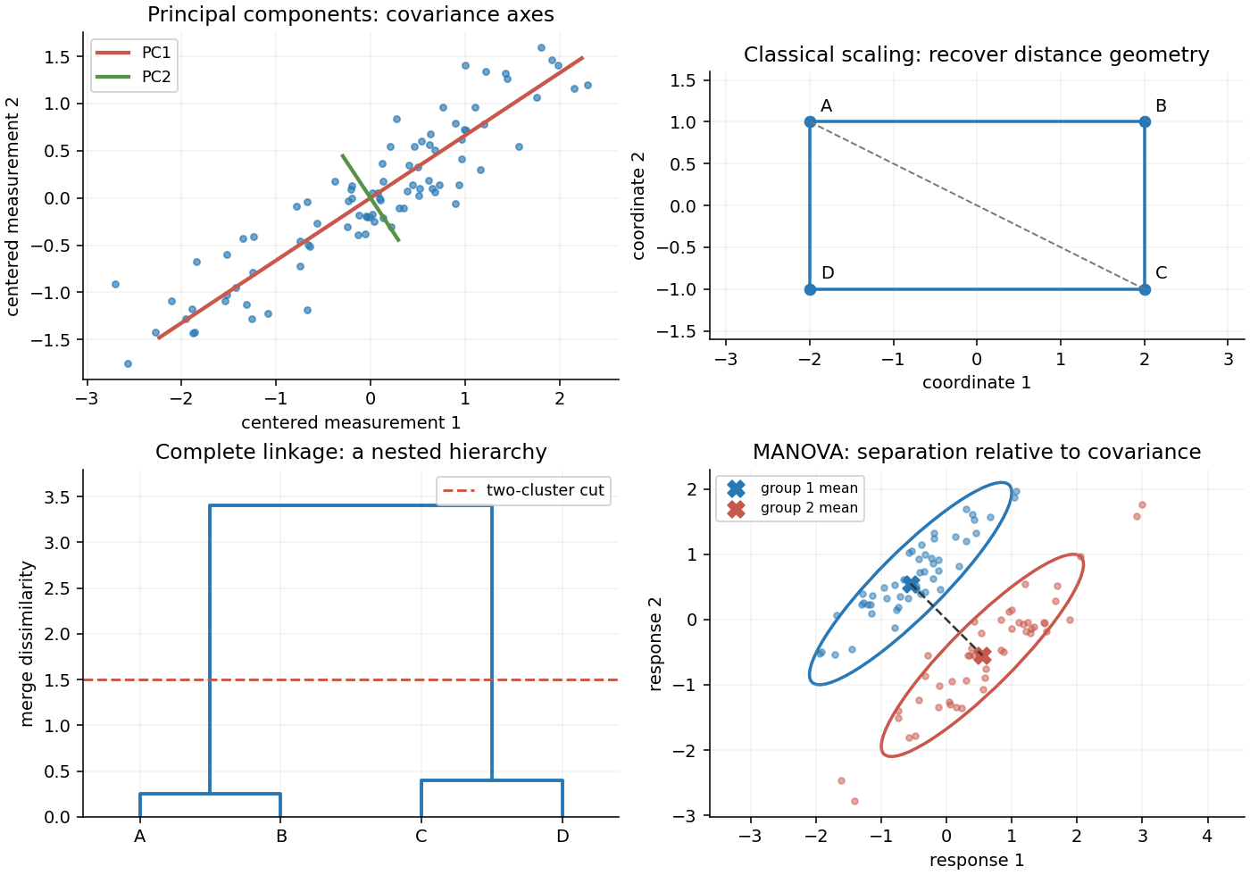
Original sketches of principal components, classical scaling, hierarchical clustering and multivariate mean comparison
. Details. 
These methods depend on measurement scale. A variable measured in large numerical units can dominate covariance-based principal component analysis; standardizing variables gives principal component analysis on a correlation matrix. Scores summarize patterns, but the method neither establishes causation nor guarantees that the largest-variance directions best predict a separate response.
Classical multidimensional scaling begins with a symmetric dissimilarity matrix , rather than necessarily with measured coordinates. Its aim is to find a low-dimensional Euclidean configuration representing those dissimilarities. Square the entries, not the matrix product, and defineFor centered coordinates , squared Euclidean distances satisfy with . Multiplication on both sides by annihilates the two single-index terms, proving the double-centering formula.
If is positive semidefinite, use its spectral decomposition to constructKeeping all positive eigenvalues reproduces the original Euclidean distances exactly; their number is the minimal embedding dimension. Keeping fewer gives a low-rank approximation to the Gram matrix. It minimizes squared Gram-matrix error, often called strain, rather than necessarily the sum of squared errors in raw distances. Negative eigenvalues signal that the dissimilarities cannot be represented exactly by Euclidean coordinates; discarding them produces an approximation whose adequacy should be inspected.
In the upper-right sketch, the supplied distances come from four points in a rectangle, and the two-dimensional reconstruction recovers that shape. The overall translation, rotation and reflection of the configuration are not identifiable from distances. Classical scaling reconstructs centered geometry from pairwise distances. If the input distances are computed from centered multivariate observations, classical scaling and principal component analysis give the same score configuration up to an orthogonal transformation: their matrices and share the nonzero squared singular values.
Agglomerative hierarchical clustering starts with each observation as a singleton cluster in cluster analysis, repeatedly joins the closest pair of current clusters, and continues until one remains. The input is a dissimilarity matrix, so choosing variable scales and a scientifically sensible dissimilarity is part of the analysis.
Different linkages define closeness differently:Single-linkage clustering can connect elongated chains through nearest neighbors; complete-linkage clustering emphasizes compact clusters; average-linkage clustering averages all cross-pair distances. For Euclidean observations, Ward minimum-variance clustering instead chooses the smallest increase in within-cluster squared error,This follows by expanding squared deviations around the merged mean and using the zero sums of within-cluster residuals.
A dendrogram plots merge heights. In the lower-left sketch, two close pairs first merge at small heights, then join across a much larger separation; a horizontal cut between these heights yields two groups. The hierarchy gives nested partitions, not a uniquely established number of populations. Examine sensitivity to scaling, linkage and ties; once an agglomerative merge is made, the method does not undo it. The absence of a probability model also means that a visually attractive dendrogram is not itself a significance test.
Multivariate analysis of variance tests differences between group mean vectors when each experimental unit has several correlated responses. For independent -dimensional observations in groups, use a common positive-definite covariance matrix and the multivariate normal model . The null hypothesis is equality of all means.
Write , group means , and the size-weighted grand mean . The within-group and between-group scatter matrices areExpanding deviations about the group means yields total scatter , with zero cross terms. Under the null, orthogonal normal projections give independent Wishart distributions and .
With nonsingular , the Wilks lambda statistic iswhere the nonnegative are eigenvalues of . Maximizing the common covariance under the two mean models gives the likelihood ratio , so small indicates large group separation relative to within-group spread. For fixed and large group sizes, the Wilks theorem gives under the null; a finite-sample reference distribution can also be used.
The lower-right sketch shows two elongated groups whose centroid difference lies nearly across, rather than along, their long axes. Their correlation makes this multivariate separation much clearer than either marginal mean shift alone. Nonsingular linear rescaling changes and by congruence, leaving the determinant ratio unchanged. MANOVA measures mean separation against the full within-group covariance geometry. Its interpretation requires independent observations and an adequate common-covariance model; separate coordinatewise tests discard that geometry and raise multiple-testing issues.
A balanced incomplete block design has treatments and blocks, each containing distinct treatments with . Every treatment occurs in blocks and every distinct treatment pair occurs together in blocks. A symmetric balanced incomplete block design has , which implies by the first counting identity below.
For the separate even-order condition, let be the square treatment-by-block incidence matrix of a set system of a symmetric design. Its diagonal overlap counts are and its off-diagonal counts are , givingThe counting identities proved in the next slots show that and . Consequently the eigenvalues of are on the constant vector and on its -dimensional orthogonal complement. Taking determinants givesIf is even, the exponent is odd. The exponent of every prime in and in is even; therefore its exponent in the positive integer must be even. This proves the even-order symmetric design square obstruction:It is a necessary condition, not a sufficiency claim.
Count incidences of a treatment with a block containing it. Summing over blocks gives , while summing over treatments gives . Hence the balanced incomplete block design satisfies
Fix one treatment. Each of its blocks supplies companion treatments, giving incidences. Alternatively, each of the other treatments accompanies it in exactly blocks. Thus
Let be the incidence matrix of a set system. The balanced incomplete block design overlap counts give . On the zero-sum subspace its eigenvalue is ; on the constant vector its eigenvalue is . Therefore has matrix rank . Since a product cannot have larger rank than either factor,This proves Fisher's inequality for block designs directly. The incomplete, nontrivial hypotheses ensure the positive eigenvalue needed for this argument.
Symmetry forces , and the pair-counting identity becomes . Its only positive integral solution is . Since the number of blocks is even, the even-order symmetric design square obstruction requires to be a square. It is not. No design with these parameters exists.
The identities require and , so . Take treatments and the four blocksEach treatment is absent from exactly one block, hence occurs three times. Each pair is absent from the two blocks missing one of its members, hence occurs together in the other two. This is the required symmetric balanced incomplete block design; here is indeed a square.
Code the two levels of each factor as . For a factor subset , its factorial contrast column is the character . Products of columns correspond to symmetric differences of subsets, because .
Let be defining words whose incidence vectors are linearly independent over . Write , with . Specifying signs is then a rank- system of binary linear equations. Every one of its right-hand sides has solutions. Thus independent defining contrasts split the full design into equal fractions. Independence is necessary: dependent defining words do not yield distinct sets.
The defining contrast subgroup has words. On a selected fraction its word has a constant sign , soHence the coefficients of and cannot be estimated separately without assumptions or extra runs: this is aliasing in a fractional factorial design. Conversely, averaging a character over the affine binary solution space vanishes unless its word is in the defining subgroup, so these signed subgroup cosets give all aliases. Here a lowercase treatment label records the factors at their high levels, and puts all five at their low levels; signs must be retained when listing aliases.
On these eight runs, and . The two independent defining words therefore give the full signed defining relationMultiplying each desired factorial contrast by its four words gives all aliases. In the following equalities a minus sign means opposite contrast columns:Thus two main effects, and , are inseparable even when every unwanted interaction vanishes. In addition, the important interaction aliases with the main effect . Design (a) is unsuitable. The seven-column design matrix for the intercept, the five main effects and has rank five, confirming the two independent estimability failures.
For this fraction, and , so their product is . The signed defining relation isThe complete factorial contrast alias classes areThe five main effects and occupy six distinct alias classes, and none aliases with the intercept. Every undesired two-factor term in these classes is assumed negligible, and all terms of order at least three are also assumed negligible. Thus design (b) is suitable under the stated interaction assumptions. Its intercept and six requested columns are mutually orthogonal, with , so each coded regression coefficient is . The corresponding high-minus-low main effect is .
There is one residual degree of freedom, but no replicated setting and therefore no separate pure error estimate. Suitability here means estimability under the stated model; it does not protect estimates from active interactions that the assumptions exclude.
For the general normal linear model, minimizing gives the least-squares normal equations . Full column rank makes invertible, soThe mean and covariance follow by substituting and using , . Normal errors also give the exact multivariate normal distribution of this estimator.
Use coded experimental variablesTheir origin is the middle of the allowed rectangle, and the stated endpoints become . The four corners and center runs give mutually orthogonal columns , withWriting when , the ordinary least squares estimates areTheir variances are , , , with zero covariances.
The repeated center runs estimate pure error without requiring the fitted mean surface to be correct:They also permit a center-point curvature contrast. Let and . Under the first-order model, and . Under a quadratic surface, its expectation is , since the linear and terms average to zero. Thusunder the first-order normal model. With only one center run there is no pure-error degree of freedom. A zero center contrast does not exclude all curvature, because the two quadratic coefficients can cancel. The corners also estimate an interaction contrast; the full Lack-of-fit F-test compares the first-order fit with the five setting means, with two lack-of-fit and pure-error degrees of freedom.
If the first-order model is adequate and , steepest ascent in response surface methodology uses the unit coded direction . The Cauchy-Schwarz inequality proves that it maximizes the predicted directional derivative. Run sequential settings for increasing feasible , corresponding to physical increments from the center. Stop or reduce the steps when measured yield ceases to improve, and refit locally near promising settings. Respect the allowed rectangle; if a boundary is reached, investigate feasible boundary directions rather than extrapolating outside it. A near-zero gradient offers no first-order ascent direction and calls for further modeling.
If curvature is indicated, add the four axial settings , together with further center replication. This face-centered central composite design stays inside the allowed physical ranges and separates the two squared coordinates, which the corners alone cannot do. Fit the full quadratic regression surfaceWrite its fitted quadratic part as , where , and . Its gradient and Hessian are and . If is nonsingular, the stationary setting isIf is negative definite and is feasible, it is the fitted maximum. Otherwise compare feasible stationary settings, optima on each edge obtained from the restricted one-variable quadratic, and the corners. A singular or poorly determined calls for attention to ridge directions and more runs. Convert any chosen coded setting back using , , and confirm its yield experimentally. The fitted local surface guides the search; it does not establish an untested physical optimum.
Articles by others on the same topic
There are currently no matching articles.