Principal component analysis replaces correlated measurements by orthogonal linear coordinates ordered by their variance. For centered observations collected in an matrix , write the sample covariance matrix as . A unit loading vector gives score vector with sample variance . The Rayleigh quotient is maximized by a unit eigenvector of for its largest eigenvalue.
The subsequent principal components maximize the same quadratic form subject to orthogonality to the earlier loading vectors. By the spectral theorem, if with descending eigenvalues, the scores have diagonal covariance . Their fractions of explained variance are . Repeated eigenvalues identify an eigenspace rather than a unique axis.
Keeping the first principal components gives the rank- reconstruction . Its squared reconstruction error isFor any rank- orthogonal projection , retained variance is . The weights lie in and sum to , so this is at most the sum of the largest eigenvalues. Projecting onto any candidate reconstruction subspace is its best least-squares reconstruction; this proves the minimum-error property and agrees with the singular value decomposition. Thus PCA finds the linear subspace preserving the greatest variance, equivalently minimizing squared reconstruction error. The upper-left sketch shows the first axis aligned with the elongated cloud; the second is perpendicular. A scree plot and substantive interpretability help choose .
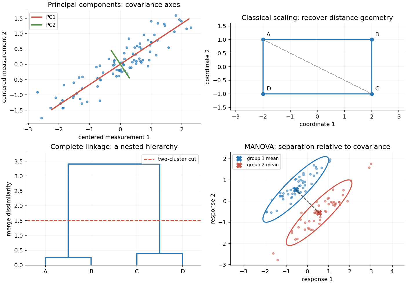
Original sketches of principal components, classical scaling, hierarchical clustering and multivariate mean comparison
. Details. 
These methods depend on measurement scale. A variable measured in large numerical units can dominate covariance-based principal component analysis; standardizing variables gives principal component analysis on a correlation matrix. Scores summarize patterns, but the method neither establishes causation nor guarantees that the largest-variance directions best predict a separate response.
Classical multidimensional scaling begins with a symmetric dissimilarity matrix , rather than necessarily with measured coordinates. Its aim is to find a low-dimensional Euclidean configuration representing those dissimilarities. Square the entries, not the matrix product, and defineFor centered coordinates , squared Euclidean distances satisfy with . Multiplication on both sides by annihilates the two single-index terms, proving the double-centering formula.
If is positive semidefinite, use its spectral decomposition to constructKeeping all positive eigenvalues reproduces the original Euclidean distances exactly; their number is the minimal embedding dimension. Keeping fewer gives a low-rank approximation to the Gram matrix. It minimizes squared Gram-matrix error, often called strain, rather than necessarily the sum of squared errors in raw distances. Negative eigenvalues signal that the dissimilarities cannot be represented exactly by Euclidean coordinates; discarding them produces an approximation whose adequacy should be inspected.
In the upper-right sketch, the supplied distances come from four points in a rectangle, and the two-dimensional reconstruction recovers that shape. The overall translation, rotation and reflection of the configuration are not identifiable from distances. Classical scaling reconstructs centered geometry from pairwise distances. If the input distances are computed from centered multivariate observations, classical scaling and principal component analysis give the same score configuration up to an orthogonal transformation: their matrices and share the nonzero squared singular values.
Agglomerative hierarchical clustering starts with each observation as a singleton cluster in cluster analysis, repeatedly joins the closest pair of current clusters, and continues until one remains. The input is a dissimilarity matrix, so choosing variable scales and a scientifically sensible dissimilarity is part of the analysis.
Different linkages define closeness differently:Single-linkage clustering can connect elongated chains through nearest neighbors; complete-linkage clustering emphasizes compact clusters; average-linkage clustering averages all cross-pair distances. For Euclidean observations, Ward minimum-variance clustering instead chooses the smallest increase in within-cluster squared error,This follows by expanding squared deviations around the merged mean and using the zero sums of within-cluster residuals.
A dendrogram plots merge heights. In the lower-left sketch, two close pairs first merge at small heights, then join across a much larger separation; a horizontal cut between these heights yields two groups. The hierarchy gives nested partitions, not a uniquely established number of populations. Examine sensitivity to scaling, linkage and ties; once an agglomerative merge is made, the method does not undo it. The absence of a probability model also means that a visually attractive dendrogram is not itself a significance test.
Multivariate analysis of variance tests differences between group mean vectors when each experimental unit has several correlated responses. For independent -dimensional observations in groups, use a common positive-definite covariance matrix and the multivariate normal model . The null hypothesis is equality of all means.
Write , group means , and the size-weighted grand mean . The within-group and between-group scatter matrices areExpanding deviations about the group means yields total scatter , with zero cross terms. Under the null, orthogonal normal projections give independent Wishart distributions and .
With nonsingular , the Wilks lambda statistic iswhere the nonnegative are eigenvalues of . Maximizing the common covariance under the two mean models gives the likelihood ratio , so small indicates large group separation relative to within-group spread. For fixed and large group sizes, the Wilks theorem gives under the null; a finite-sample reference distribution can also be used.
The lower-right sketch shows two elongated groups whose centroid difference lies nearly across, rather than along, their long axes. Their correlation makes this multivariate separation much clearer than either marginal mean shift alone. Nonsingular linear rescaling changes and by congruence, leaving the determinant ratio unchanged. MANOVA measures mean separation against the full within-group covariance geometry. Its interpretation requires independent observations and an adequate common-covariance model; separate coordinatewise tests discard that geometry and raise multiple-testing issues.
Articles by others on the same topic
There are currently no matching articles.