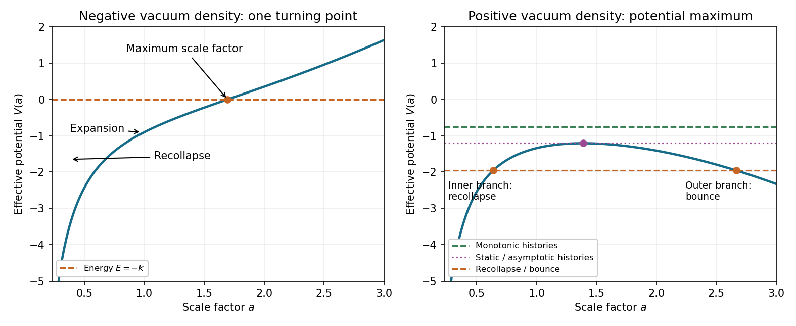
Use cosmic time here; derivatives with respect to conformal time will be used from Question 2 onward. Conservation of pressureless matter and radiation in cosmology makes and constant. DefineThe Friedmann equation is a mechanical energy equation,For nonnegative dust and radiation, at least one nonzero, tends to as and to as , whileThus every energy line meets the potential once. An expanding solution reaches this turning point and then contracts: . The Friedmann effective potential for matter, radiation and vacuum is sketched below, alongside the positive-vacuum case.

To bound the full cosmic time from the initial zero of to its final zero, use the Friedmann acceleration equation:Put maximum expansion at , with and . The forced-oscillator identity isUntil the first zero and for , the kernel is nonnegative and the bracket is nonpositive. Hence , so contraction cannot remain at positive beyond . Applying the same argument backward from maximum expansion bounds the expanding half. Therefore the negative-vacuum Friedmann lifetime bound isAt either endpoint, nonzero dust or radiation has divergent density. If both are absent, the same estimate instead bounds the open Anti-de Sitter spacetime coordinate patch; its coordinate zeros are not a finite lifetime of the maximally extended vacuum spacetime.
Set . The Friedmann effective potential for matter, radiation and vacuum now readsWith nonzero nonnegative dust or radiation, tends to at both ends. Its stationary point satisfiesEquivalently when ; the right-hand side decreases strictly, so there is exactly one stationary point. It is a maximum becauseThe energy line in the preceding sketch therefore gives five broad types of history:
- Monotonic expansion. For , the universe expands from to arbitrarily large .
- Monotonic contraction. Reversing cosmic time gives the corresponding contracting history.
- Recollapse. For , the inner allowed interval ends at : the universe expands from zero to and contracts back to zero.
- Bounce. The outer allowed interval starts at . A universe contracting from large reaches and re-expands. Here , so at the turning point.
- Static equilibrium. For , and give the Einstein static universe.
At the critical energy there are also marginal branches within the monotonic classes: expansion from zero can approach asymptotically, or expansion can start asymptotically at and proceed to infinity; contraction gives their reversals. They must not be mistaken for reaching the static solution in finite time. Indeed near the maximum,so diverges logarithmically. The static equilibrium is unstable. Since , the recollapsing, bouncing and static cases require positive spatial curvature .
For an Einstein static universe, both and vanish. The Friedmann acceleration equation givesand therefore impliesThe Friedmann equation additionally fixes the spatial curvature:Thus the acceleration balance is necessary but must be accompanied by the static energy constraint.
Without radiation, the Friedmann acceleration equation changes sign when . The cosmological redshift satisfies , and conservation of pressureless matter gives . HenceThe expanding spatially flat model is decelerating above this redshift and accelerating below it. Positive is required for such a transition; a negative value gives no accelerated expanding epoch. If the displayed redshift is negative, the transition lies in our future.
Write , where primes denote conformal time. In the passive convention for a cosmological gauge transformation, retain terms linear in or and discard their products. The linear metric gauge-transformation law then givesFor a single nonzero Fourier mode, suppress the common factor . Its derivatives areUsing and therefore yieldsThe term proportional to comes from the time dependence of the background scale factor; omitting it would transform only the flat reference metric.
For the synchronous-to-Newtonian scalar Fourier transformation, the coefficient of in the transformed spatial metric perturbation must vanish. Thus . Vanishing shift then gives . For these conditions fixThe lapse in conformal Newtonian gauge is , soThe remaining coefficient of isgivingThe homogeneous perturbation requires separate background-coordinate choices; the inverse powers of do not define a transformation for it.
Preserving synchronous gauge means and . The first equation is , and integration of the second gives the complete residual scalar transformation for each nonzero Fourier mode:Changing the lower limit only changes . Taking the trace and trace-free longitudinal part of givesConsequently and . The cosmological Newtonian potential changes bywhile its spatial counterpart changes byThus both potentials are invariant under residual synchronous-gauge freedom, although and individually are not.
During matter domination, the spatially flat background has and . Let denote the scalar velocity divergence. Linear stress-energy conservation in synchronous gauge givesThe first equation follows from the perturbed volume element ; the second states that peculiar dust velocity redshifts as . Differentiating the first and substituting the trace of the Einstein field equations, with and , yieldsThereforeTrying gives . The complete solution of this density equation isThese are the matter-era growing and decaying density modes, proportional to and . In a dust-comoving synchronous gauge, and . That rest-frame choice distinguishes physical mode coefficients from changes of density induced by residual synchronous-gauge freedom.
Define the matter power spectrum by the Fourier transform conventionStatistical isotropy then givesFor the growing mode found above, write . At cosmological horizon entry, , so the variance contribution per logarithmic interval is proportional to . Making it independent of requires . HenceThis is the Harrison-Zeldovich spectrum. Scale invariance applies at horizon entry, not to the unprocessed density variance on a common late-time slice. In the notation , it means , with random Fourier coefficients supplying the ensemble statistics.
Neglecting the rapidly oscillating radiation source on subhorizon scales, stress-energy conservation and the trace of the Einstein field equations giveEquivalently in cosmic time, . Radiation still contributes to the background expansion, even when its perturbation source is averaged away.
Put and let be the density of either component at matter-radiation equality. Then and . With , the Friedmann equation givesApply the chain rule to the density equation:Thus the Mészáros equation isSubstituting gives , sois indeed a solution. It is approximately constant during radiation domination and grows as during matter domination. The second independent solution iswhich behaves as at small . Thus smoothing radiation does not eliminate every logarithmic solution; matching through actual horizon entry fixes the combination excited.
Modes with enter after equality and retain the shape. Modes with enter during radiation domination: their horizon-entry spectrum is and they gain little growth until equality. The late matter power spectrum therefore turns over near and has a large-scale branch and a small-scale branch, with the more accurate radiation-era matching givingEquivalently the cold-dark-matter transfer function falls approximately as , up to the logarithm. The turnover is the consequence of the Mészáros effect; it is not a change of the primordial scale-invariance condition.
The emission term comes from the local photon temperature. A blackbody radiation density is proportional to , so linearization gives . It is evaluated at last scattering, with the source position on the observed ray.
The velocity term is the Doppler CMB anisotropy: motion of the emitting plasma changes the measured photon frequency by the component of its peculiar velocity along the line of sight. Its sign here follows the paper's choice of the sky direction .
The metric integral follows the null geodesic energy equation in synchronous gauge. Time dependence of the spatial metric perturbation changes the photon energy by along the ray. It includes gravitational redshift endpoint terms as well as the part due to evolving gravitational potentials. In particular, the entire synchronous metric integral is not just the integrated Sachs-Wolfe effect. Integrating by parts to express it in conformal Newtonian gauge separates the ordinary Sachs-Wolfe effect from the evolving-potential contribution.
Use one Fourier mode, with and unperturbed ray . Put , and let denote last scattering. In the supplied branch , the scalar decomposition givesSince , two integrations by parts give the exact endpoint decomposition of the metric contribution:For the matter-era growing mode, is quadratic in , so the last integral vanishes. With , the emission endpoint isand the observer endpoint is . The observer terms are only a angular monopole and angular dipole; they are removed when studying the anisotropy multipoles .
For an adiabatic growing mode outside the horizon at last scattering, , after fixing the constant trace convention, and . Hence the intrinsic emission term is smaller than by order . The derivative emission endpoint is smaller by order . Stress-energy conservation also makes the peculiar emission velocity subleading; its leading synchronous contribution cancels in , with gradients supplying the remaining small term. Keeping the Fourier phase, which need not be small over the observer's distance, givesHere , and the sum over modes is understood. The derivative is the second derivative of , as printed in the original PDF. This approximation assumes matter-era growing adiabatic modes and neglects late evolving potentials; large wavelength alone does not remove the last integral in a general cosmology. The equality is used as the supplied synchronous condition, rather than as a general identity for every fluid solely from vanishing anisotropic stress.
Write the growing density contrast as , with having the indicated spectral amplitude. In the dust-comoving synchronous gauge, , and the supplied therefore implies . On the same comoving density slicing, the cosmological Poisson equation isbecause . This is the comoving-density form of the relativistic scalar constraint, so it can be used on these large scales; replacing its density by the Newtonian-gauge density would not be justified there. Combining the two results givesThus the large-angle Sachs-Wolfe effect has source . The potential is constant for this matter-era growing mode, and its power spectrum obeys .
Restore the Fourier transform integral and the last-scattering distance:Insert the Rayleigh plane-wave expansion and use orthogonality of spherical harmonics with the complex conjugate on the projection harmonic. The angular integral selects the matching indices, givingThe complex conjugation is present in the original PDF. If denotes a mode coefficient with its random amplitude and phase included in , substitution of gives the equivalent factor inside the Fourier integral. The monopole and local observer dipole removed in part (b) do not change this formula for .
Let . Statistical isotropy and applied to the preceding expression give the CMB angular power spectrumFor , define the constant dimensionless potential power . ThenThe needed logarithmic spherical Bessel square integral can be proved directly. Put and . From the Spherical Bessel function recurrences,integration of the squares' derivatives gives , and for also . At , and give , hence . Induction now proves . ConsequentlyThis is the flat large-angle Sachs-Wolfe plateau. The useful integral printed in the PDF is missing the square on : without that square the formula is false, since at its left-hand side is , whereas its asserted value would be . The squared identity above is the one required by the variance calculation. The plateau describes the matter-era large-angle approximation, not acoustic peaks or late integrated-potential corrections.
Introduce conformal timeIt satisfies and , so the metric becomes . Choose null coordinatesThus is positive on . Choosing the two null coordinates with these orientations gives the requested positive coefficient of .
There is a global-topology distinction in the source: unrestricted gives the universal cover of two-dimensional de Sitter spacetime. The usual two-dimensional de Sitter spacetime has periodic modulo . Indeed its standard embedding is , , , and is unchanged by . The local metric and the null-coordinate calculation apply to either choice.
The positive conformal factor leaves the causal structure unchanged. In the strip , a future-directed causal curve obeysand null geodesics have slopes . Its past and future conformal boundaries are spacelike. A finite conformal time interval limits the range of light signals: the observer at can receive a signal from before future infinity exactly when . Equality describes its observer-dependent cosmological event horizon.
For a finite Penrose diagram of the unwrapped spatial coordinate, set , , , and . Then the metric is conformal to ; light rays remain at degrees, and the boundaries are the images of . The figure also shows the spatially periodic de Sitter cylinder so that the global distinction is explicit.
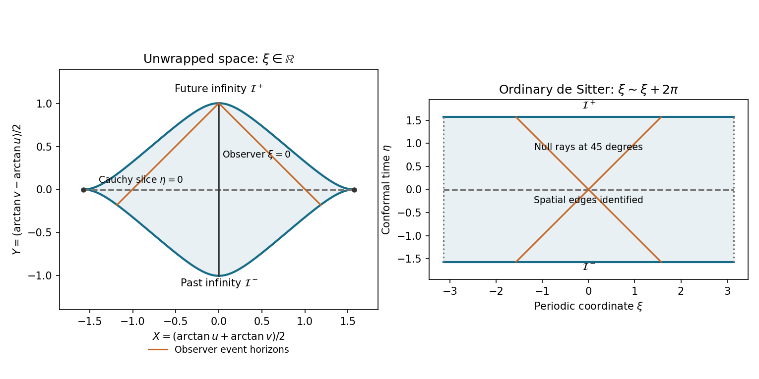
Causal compactification of the unwrapped de Sitter strip and the spatially periodic de Sitter cylinder
. Details. 
Both the covering spacetime and the de Sitter cylinder are globally hyperbolic. To see this directly in the covering spacetime, suppose an inextendible future-directed causal curve had a future limiting conformal time strictly below . The slope bound makes Cauchy as that time is approached, so the curve has a limiting point inside the spacetime and can be extended, a contradiction. The past endpoint similarly approaches . Thus every constant- line is crossed exactly once and is a Cauchy hypersurface. On the cylinder the same argument uses compactness of the spatial circle. Equivalently causal diamonds between finite events are bounded and closed within the strip, hence compact.
Initial field data on a complete Cauchy hypersurface determine a unique solution for a well-posed hyperbolic Cauchy problem, with the relevant constraints imposed for constrained systems. Spacelike conformal infinity does not require additional timelike-boundary conditions. An observer's cosmological horizon limits which data that observer can see; it does not destroy global uniqueness from data on the whole hypersurface.
Vary the action with compactly supported variations and integrate by parts. Its overall normalization does not affect the equation of motion:Here , so the massless scalar field obeysSeparate a spatial Fourier mode as . Its mode equation is . With conformal time , and , it becomesFor , put and . Direct differentiation reduces the equation tothe Spherical Bessel function equation with order one. Hence the complete classical mode basis isSince and , an equivalent complex basis isThe classical action does not select one frequency branch or a quantum vacuum. A real field has conjugate-related coefficients at opposite wavevectors. The zero mode, which is not obtained by treating these two basis functions as independent at , isAt late times one independent solution freezes and the other decays as . These are minimally coupled massless modes; the supplied action has no curvature-coupling term, so it should not be replaced by the conformally coupled wave equation.
Normalize a point source by on the compact spatial direction. The periodic delta has the Fourier seriesWriting the potential as reduces the Poisson equation toAway from the source, the decaying radial solution is proportional to . Its distributional normalization follows from integrating the Laplacian over a small sphere: the radial flux of is , soThis is the contribution of the th Kaluza-Klein mode, with inverse range . At equal compact coordinate, the sum is a geometric series,Therefore the pair interaction energy, without the individual self-energies, isIts normalization is fixed by the stated source, rather than by importing another convention for Coulomb's law. More generally summing the phases gives the periodic electrostatic Green function with one compact dimension,An independent check uses the method of images in four spatial dimensions. Since , its periodic image sum is , with the same normalization and short-distance singularity.
For , only the zero Kaluza-Klein mode survives:For , givesThe leading potential thus changes from inverse distance to inverse squared distance. Differentiating gives the signed outward forceIt scales as at large distance and as at small distance. A precision inverse-square-law test over separations approaching would reveal the extra dimension through this change of force law or its exponential corrections. The model assumes localized sources at equal compact coordinate and an electromagnetic field able to explore the circle; a field confined to ordinary spacetime would not show this effect. Finite source size and ordinary screening must be controlled when comparing a real force measurement with this point-source prediction.
Articles by others on the same topic
There are currently no matching articles.