For , polar coordinates give and ; the remaining amplitude equation is . Interpret in the original complex coordinate, where the phase is undefined.
If , put . The full equilibrium points are . Their eigenvalues areThus is stable for and has a two-dimensional unstable manifold for . The point has a one-dimensional unstable manifold for and is repelling for . On they merge in a saddle-node bifurcation; the simultaneous zero and imaginary eigenvalues at give a fold-Hopf bifurcation.
A steady positive amplitude represents a full periodic orbit, not a full equilibrium. Solving the amplitude equations givesIt exists in the wedge . The transverse amplitude Jacobian matrix has characteristic polynomial . Its two transverse Floquet exponents have negative real part for and positive real part for ; the phase direction supplies the neutral Floquet multiplier one.
The wedge boundaries are Hopf bifurcations at from and from . The left branch is supercritical, producing a stable periodic orbit as loses stability; the right branch is subcritical in the oscillatory subspace, with an unstable periodic orbit on the side where the transverse complex pair of is stable. The real unstable direction of persists throughout. There are no full equilibrium points when , and then excludes a local periodic orbit. The right panel of the bifurcation diagram in part 1(b) shows the primary curves and the perturbed global curve calculated below.
Within the positive-amplitude wedge the reduced periodic orbit equilibrium has amplitude trace and positive determinant . At the transverse pair is imaginary, so the possible secondary event is a Hopf bifurcation of the amplitude equations, corresponding to an invariant torus in the full system.
It is degenerate. Set and . The first integral of the quadratic fold-Hopf amplitude flow isThe amplitude equations have the Hamiltonian system form , , so . At , has a strict local maximum and negative-definite Hessian. Every nearby regular level is a closed amplitude periodic orbit, rather than one isolated orbit selected by nonlinear damping. Adding the rotating phase gives an entire family of invariant tori; the full motion is quasiperiodic or periodic according to the phase advance during one amplitude period.
For , the amplitude vector field has constant divergence . The Bendixson-Dulac theorem rules out closed amplitude trajectories in the physical simply connected half-plane . Hence there is no ordinary branch of isolated invariant tori on either side in this quadratic system. The secondary event has vanishing radial saturation coefficients; its imaginary linear pair alone does not establish a nondegenerate torus bifurcation.
With the added term, , while and . The prescribed rescaling yieldswhere primes denote . In the limit , the first integral is , since , .
Write . The physical amplitude half-plane is , with of either sign; it is the radial variable , not the axial variable , that is nonnegative. The centre equilibrium is , at . The boundary saddle equilibria are , both at . For , the contours are nested closed curves around the centre. The level consists of the boundary and the interior arcOn the axis , giving a heteroclinic orbit from to . On the arc , giving the reverse heteroclinic orbit. Together they form a heteroclinic cycle. The other parts of the zero level and negative levels give nonclosed trajectories outside this bounded region. The requested contour sketch is shown in the physical radial half-plane.
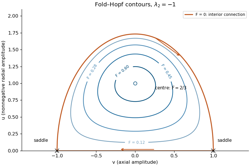
Conserved amplitude contours and the heteroclinic cycle of the quadratic fold–Hopf system
. Details. 
For the perturbed amplitude equations, direct differentiation of the first integral givesThe axis connection contributes zero since . On the unperturbed interior heteroclinic orbit, and , so the first-order change isThe substitution givesConsequentlyThe simple zero of this Melnikov energy-balance method calculation gives the heteroclinic splitting of a fold-Hopf amplitude cycle:This is a leading persistence curve, not an exact parameter equality for the perturbed orbit. It lies between the two primary Hopf bifurcation curves near the origin and on the negative- side of the secondary torus curve . With the added term the primary Hopf bifurcation curves themselves shift to .
The sign of the amplitude balance also identifies the local torus branch. Over a small closed limiting contour, . Its enclosed-area form sets equal to minus the area-average of . This average tends to zero at the centre and to at the heteroclinic cycle. Near the centre, negative attracts trajectories toward the stable amplitude equilibrium; outside a zero-balance contour, decreases and the amplitude excursion grows. Thus the secondary bifurcation creates an unstable invariant torus on the stable-periodic-orbit side. Its continuation reaches the global connection as the balance tends to . The bifurcation diagram distinguishes this perturbed connection from the entire degenerate family present in the unperturbed system.
The normal form is invariant under . This continuous rotational symmetry makes the axis invariant and reduces the nontrivial geometry to two amplitude variables. The axis connection from to persists without parameter tuning, while rotating the outer connection produces a family of connections from back to . A two-dimensional autonomous amplitude flow cannot by itself produce the proposed saddle-focus return chaos: symmetry reduction hides the phase-dependent reinjection needed for that mechanism.
Generic higher-order terms need not retain this exact rotational symmetry. A normal form can preserve it to a finite truncation order while the full equations have small symmetry-breaking remainders. These unfold the special connection geometry into phase-dependent returns; nearby parameter curves can contain homoclinic orbits to a saddle-focus, and the Shilnikov bifurcation mechanism becomes available. Their exact placement depends on the omitted terms and is not fixed by the displayed truncation alone.
For example, at the perturbed positive-axis saddle, the real unstable eigenvalue is and the stable complex pair has real part . Near the calculated connection curve , the contracting ratio isThis is the positive-saddle-value regime, explaining why the relevant saddle-focus return can be expanding.
In the Shilnikov return map, take a positive return coordinate and , with nondegenerate . At the connection parameter , the fixed point condition isThe right side tends to zero, whereas the phase passes through infinitely many oscillations as . Hence there are infinitely many positive fixed points accumulating at zero, with logarithmically spaced amplitudes. For these points,whose magnitude tends to infinity along the accumulating fixed-point sequence. They represent long-period saddle periodic orbits of the full return, with period growing like , rather than infinitely many stable cycles.
Successive turning branches of this oscillatory return can stretch and fold across suitable intervals. The full saddle-focus Poincaré return map then admits invariant Smale horseshoes and chaotic itineraries near a generic homoclinic orbit at a Shilnikov bifurcation. Varying unfolds accumulating saddle-node and period-doubling events. Whether any resulting invariant set attracts trajectories depends on the other return direction and the omitted terms; the leading scalar map alone does not prove a chaotic attractor for every perturbation. Its domain also excludes negative iterates, which leave the chosen return branch. The degeneracies or would remove the oscillatory mechanism, so the conclusion uses generic, genuinely saddle-focus reinjection.
Articles by others on the same topic
There are currently no matching articles.