Past exam of the mathematics course of the University of Cambridge / 2004 / iii / Paper 77 (Fluid Mechanics of Swimming Organisms)

The Lighthill elongated-body theory approximation treats each cross-section of a slender swimmer as a locally two-dimensional potential flow problem. The transverse dimension is small compared with the length and the scale over which cross-sections vary. The displacement and slope are small enough to linearize the impermeability condition about a straight body. The Reynolds number is sufficiently large for lateral loading to be dominated by fluid inertia; viscosity, axial friction and higher-order end corrections are neglected at this order. This reactive approximation must be distinguished from the viscous resistive-force theory used for a flagellum.

In coordinates translating with the swimmer, the undisturbed fluid passes in the positive $x$ direction at speed $U$. Applying the impermeability condition to the moving centre plane gives the transverse fluid velocityThe local added mass $m(x)$ is defined so that the transverse fluid hydrodynamic impulse per unit axial length is $P_y=m(x)v_y$. A fixed body-coordinate interval receives an impulse flux $U{P}_y$ at its leading end and loses the corresponding flux at its trailing end. Its rate of change of impulse plus the net outward impulse flux is thereforeThis is the transverse force exerted by the body on the fluid. By Newton's third law, the transverse force exerted by the fluid on the body has the opposite sign:The distinction is essential here: the printed positive expression is labelled as the force on the fish, so that label and expression are inconsistent. For example, take a uniform cross-section and a rigid lateral displacement $h=H(t)$. The swimmer must accelerate fluid of added mass $m$, which reacts on it with force $-m{H}^{\prime \prime }$, not $+m{H}^{\prime \prime }$. Thus the positive expression is recovered exactly with the force-on-fluid convention; the physically consistent force on the fish is the negative expression. In the following parts, $F_y$ denotes $F_{\mathrm{body}}$ so that the beam balance uses a genuine external force on the fish.

Choose the internal transverse force $S(x,t)$ so that the net internal transverse force on a slice is $[S(x+dx,t)-S(x,t)]$. Its linear momentum balance is thenThe coordinate $x$ labels body slices, so their lateral material acceleration is $h_{tt}$; the fluid transport operator $\mathcal{D}$ must not be substituted for this body acceleration.

Let $G$ be the total internal bending moment, including both passive elastic and active muscular contributions. With the compatible moment orientation, the net couple on the slice is $(G_x-S)dx$. The cross-sectional rotary inertia is smaller than the translational inertia by the square of the transverse-to-longitudinal length ratio, and is neglected in this slender-beam approximation. Slice angular momentum balance therefore gives $S=G_x$. Eliminating $S$ from the slice linear momentum balance provesThis equation is the balance law for an active bending beam for a swimming fish; a constitutive relation for the passive bending moment or the muscle actuation is not needed to derive it. With the force-on-body convention established above it becomesAs a check, constant $m$ and rigid lateral acceleration give the effective inertia $m_b+m$. Combining the printed positive force in part (i) with the minus sign in the beam equation would instead give $m_b-m$. That is the same sign defect, rather than a negative hydrodynamic added mass. If the positive quantity in part (i) is called $F_y$ as a force on the fluid, the beam equation must contain $+F_y$.

A freely swimming body has neither an imposed end couple nor an imposed end transverse force. Its end bending moment is therefore zero, and the transverse force $S=G_x$ is also zero at both ends. These are the four free-end bending boundary conditions; they do not require the end displacement or slope to vanish.

Put $R=m_b{h}_{tt}+\mathcal{D}(m\mathcal{D}h)$, using the physically consistent sign. Integrating $G_{xx}=R$ with the two leading-end conditions givesThe two trailing-end conditions consequently requireThese free-end compatibility for a swimming beam conditions are total transverse force and torque balances. They explain why an arbitrary plausible prescribed $h$ does not suffice: two integration constants can satisfy only two end conditions unless the forcing already satisfies both compatibility integrals.

The missing freedom is the swimming recoil correction. An observed or prescribed deformation $h_d$ relative to the body must be supplemented by a lateral translation $Y(t)$ and a small yaw $\Theta (t)$:To identify $Y$ with the actual centre of mass displacement, first remove the body-mass-weighted mean from $h_d$. One may also remove its body-mass-weighted first moment about $x_c$ to define the yaw reference uniquely. This changes the decomposition of the observed motion, not the physical displacement.

For $\xi =x-x_c$, the recoil contribution to the forcing isInsert $R=R_d+R_{\mathrm{rec}}$ into the two compatibility integrals, using $1$ and $\xi$ as weights. This gives two coupled ordinary differential equations for the two recoil motions. Their principal acceleration matrix isFor a nondegenerate positive mass distribution it is a positive-definite matrix: its quadratic form at $(a,b)$ is ${\int }_0^L(m_b+m)(a+b\xi {)}^{2}dx>0$ unless $a=b=0$. Thus initial translation and yaw determine the recoil through these equations, and the corrected $h$ supplies the two compatibility conditions. The four free-end conditions determine the bending moment together with two rigid recoil motions; they do not overdetermine a physically complete swimming motion.

In resistive-force theory, the flagellum is slender and moves at a small Reynolds number, so local viscous resistance is linear in its velocity and fluid and body inertia are neglected. Normal and tangential resistance coefficients are treated as positive constants, usually ${\kappa }_N>{\kappa }_T$. The approximation neglects distant hydrodynamic interactions along the filament, head-tail interactions, nearby boundaries and self-contact. The centreline is an inextensible filament with prescribed shape. Its local resistance tensor isSince the filament velocity relative to distant fluid is $-\mathbf{w}$, the fluid force on a filament element is $K\mathbf{w}ds$. The equal and opposite force on the fluid has total axial component $T$. Projecting onto $\mathbf{i}$ givesThis establishes the thrust expression with its force-on-fluid convention.

For a uniform travelling wave, write the moving centreline as $\mathbf{r}(s,t)={\mathbf{r}}_{\mathrm{wave}}(s-ct)+(V-U)t\mathbf{i}$, where $s$ is material arc length and $|{\mathbf{r}}_{\mathrm{wave}}^{\prime }|=1$. Differentiating at fixed material label gives ${\mathbf{r}}_t=(V-U)\mathbf{i}-c\mathbf{t}$. HenceLet $q=\mathbf{t}\cdot \mathbf{i}=X_s$, $\alpha =⟨q⟩$ and $\beta =⟨q^2⟩$, where these brackets are contour-length averages. The axial wavelength divided by contour wavelength is $\alpha =V/c$. For a filament comprising whole wave periods, or after the usual period averaging, $c{\int }_0^{L}qds=VL$. This averaging is needed to avoid end-phase corrections for an arbitrary fraction of a wavelength. Substitution of $\mathbf{w}$ into the thrust expression now givesFor $\gamma ={\kappa }_T/{\kappa }_N$ and $r=1-\gamma$, this is $T/({\kappa }_{N}L)=Vr(1-\beta )-U(1-r\beta )$. The swimming body is force-free, so the reaction thrust on the head-tail assembly balances its head drag. Thus $T=\delta {\kappa }_{N}LU$, and linear resistive-force propulsion of a travelling filament givesWe henceforth assume $0<\gamma <1$, $\delta \ge 0$ and $0<\beta <1$. Isotropic resistance, $\gamma =1$, gives no propulsion in this model.

The flagellar contribution to viscous dissipation is the positive quadratic form $P_f=\int \mathbf{w}\cdot K\mathbf{w}ds$. Expanding it, and using $c⟨q⟩=V$, givesThere is also head dissipation $\delta {\kappa }_{N}L{U}^2$. Equivalently, the work of the flagellar deformation relative to the translating head is $P_f+UT$; the force balance makes $UT$ precisely the head dissipation. Consequently, with $\alpha =V/c$,This derives the rate of working, rather than merely inferring it from the thrust.

The Cauchy-Schwarz inequality gives ${\alpha }^2=⟨q{⟩}^2\le ⟨q^2⟩=\beta$. Equality requires $q$ to be constant almost everywhere. For a planar periodic filament this is an ideal sawtooth with alternating transverse tangent and fixed axial tangent, or a limit with negligibly rounded corners. It is not an identity for a general sinusoidal wave, and the ideal calculation omits the elastic cost of sharp corners.

For the stipulated equality ${\alpha }^2=\beta$, put $d=1+\delta$ and eliminate $V$ at fixed $U$ using $V/U=(d-r\beta )/[r(1-\beta )]$. Direct simplification yieldsThe derivative isWriting $A=r({\delta }^2-\gamma )$ and $B=\gamma d^2$, the numerator is $A{\beta }^2+2B\beta -B$. It is negative at zero and equals $(\delta +\gamma {)}^2>0$ at one. Its derivative is positive throughout $(0,1)$: this is immediate if $A\ge 0$; if $A<0$, its minimum derivative is $2(A+B)=2(\delta +\gamma {)}^2>0$. Since $F$ diverges at both endpoints, the unique stationary point is the global fixed-speed energy optimum for a planar flagellum:This form includes the case $A=0$, when ${\beta }_{\ast }=1/2$, without a removable division by zero. With no head drag it reduces to ${\beta }_{\ast }=1/(1+\sqrt{\gamma })$.

The printed final optimality formula does not follow from the preceding thrust and power equations. For a concrete check, $\gamma =1/2$, $\delta =0$ gives $F=(2-\beta )/[\beta (1-\beta )]$. The derived minimum is at $\beta =2-\sqrt{2}$. The printed formula instead gives ${\beta }^2=\sqrt{6}-2$, hence $\beta \approx 0.67044$, where $F^{\prime }\ne 0$ and the expenditure is greater. Thus the thrust and working formulas can both be established as above, but the last printed conclusion must be replaced by the derived optimum.

Neglecting cell rotational inertia, the light and viscous torque sum to zero. Therefore the angular velocity is $\mathbf{\Omega }=\mathbf{\omega }/2+(\mathbf{p}\times \mathbf{L})/\alpha$. A material orientation evolves by $\dot{\mathbf{p}}=\mathbf{\Omega }\times \mathbf{p}$. The vector triple-product identity givesThe last term is the projection of $\mathbf{L}/\alpha$ onto the tangent plane to the unit sphere. In particular, $\mathbf{p}\cdot \dot{\mathbf{p}}=0$, as required to preserve the unit orientation. It aligns the swimmer towards the light; the vorticity rotates that orientation.

For rotational diffusion coefficient $D_r$, the phototactic orientation Fokker-Planck equation balances deterministic orientation drift with diffusion on the sphere. Its density is normalized with respect to solid angle, not $d\theta d\varphi$. When $\epsilon =0$, there is no azimuthal drift and the zero-current condition is $f_{0,\theta }=-\lambda \sin \theta f_0$. Thus $f_0=\eta e^{\lambda \cos \theta }$, and normalization givesThe limiting density at $\lambda =0$ is $1/(4\pi )$.

To justify the angular dependence of the first correction, define the operatorsThe steady Fokker-Planck equation is $\mathcal{A}f=-\epsilon \mathcal{R}f$. Its regular expansion $f=f_0+\epsilon f^{(1)}+O({\epsilon }^2)$ therefore givesThe coefficients of $\mathcal{A}$ are independent of $\varphi$, so each azimuthal Fourier harmonic is preserved. The forcing has only the sine harmonic with azimuthal number one. There can be no extra unforced harmonic in a smooth normalized first correction: writing a homogeneous solution as $f_{0}h$ gives $\mathcal{A}(f_{0}h)={\nabla }_p\cdot (f_0{\nabla }_{p}h)$. Multiplication by $h$ and integration by parts on the sphere gives $\int f_0|{\nabla }_{p}h{|}^{2}d\Omega =0$, hence $h$ is constant. Normalization $\int f^{(1)}d\Omega =0$ removes that multiple of $f_0$. It follows thatNo explicit calculation of $g$ is needed. Its dependence is on $\theta$ and the parameter $\lambda$, and its behavior at the poles must make the density smooth.

In the stated spherical coordinates, $\mathbf{p}=\cos \theta {\mathbf{e}}_x+\sin \theta \cos \varphi {\mathbf{e}}_y+\sin \theta \sin \varphi {\mathbf{e}}_z$. Azimuthal integration makes the leading $y,z$ components and the first-order $x,y$ corrections vanish. The surviving coefficients areThus the small-vorticity phototactic orientation response isBoth coefficients depend only on $\lambda$. In particular, $K_0$ is the Langevin function of $\lambda$ and is positive for positive light strength; its integral representation above suffices.

The cell conservation equation equates the change of cell number density $n$ to minus the divergence of its total flux. The flux $n\mathbf{u}$ is advection by the water, $n{V}_s⟨\mathbf{p}⟩$ is the mean swimming flux, and $-\mathbf{D}\cdot \nabla n$ is the dispersal flux. The tensor $\mathbf{D}$ describes effective translational diffusion, whereas $D_r$ in part (i) describes rotational diffusion; they have different dimensions. This conservation law neglects birth, death and sources at the walls.

The equation $\nabla \cdot \mathbf{u}=0$ expresses incompressible flow. In the momentum equation, $\rho$ is the reference suspension density, $\rho [{\partial }_t\mathbf{u}+(\mathbf{u}\cdot \nabla )\mathbf{u}]$ is material acceleration times density, $-\nabla p_e$ is the pressure force after subtracting the pure-water hydrostatic pressure, and $\mu {\nabla }^2\mathbf{u}$ is the viscous force for constant dynamic viscosity $\mu$ in a Newtonian fluid. Since $n$ counts cells per volume, $g^{\prime }$ in $-g^{\prime }n{\mathbf{e}}_z$ is excess downward weight per cell; it is not an acceleration. The small cell-fluid density difference permits the Boussinesq approximation: retain that difference in buoyancy while using constant $\rho$ elsewhere. Diluteness permits neglect of cell-cell interactions, changes of viscosity, and active cell stresses. Any separate settling speed is assumed negligible or already incorporated in the specified mean drift. The light strength and swimming speed are uniform.

Consider the intended long-channel bulk approximation. At the sidewalls impose zero normal cell flux and the no-slip boundary condition. The closed ends require zero total fluid flux through each horizontal section, so ${\int }_{-a}^{a}wdx=0$; localized turning regions are omitted from the bulk equations. The mean concentration is ${\int }_{-a}^{a}ndx=2a{n}_0$. The final paragraph below distinguishes these bulk conditions from exact closed-end cell conservation.

For $\mathbf{u}=w(x){\mathbf{e}}_z$, the vorticity is $-w^{\prime }(x){\mathbf{e}}_y$. Hence $\epsilon =-w^{\prime }/(2D_r)$, and the leading horizontal mean swimming direction is $K_0{\mathbf{e}}_x$. With $\mathbf{D}=DI$ and $n=n(x)$, steady cell conservation equation says that $J_x=V_s{K}_{0}n-D{n}^{\prime }$ is constant. Its wall value is zero, so $n^{\prime }=\beta n$ with $\beta =V_s{K}_0/D$. The phototactic concentration in a vertical channel is thereforeThis result neglects the $O({\epsilon }^2)$ correction to horizontal swimming. For positive phototaxis, $\beta >0$ and cells accumulate towards the illuminated wall $x=a$.

The steady inertial terms vanish for $w=w(x)$, since $\mathbf{u}\cdot \nabla =w{\partial }_z$. The horizontal momentum equation gives ${\partial }_x{p}_e=0$. The vertical momentum equation then requires a constant excess pressure gradient $G={\partial }_z{p}_e$ and gives $\mu w^{\prime \prime }=G+g^{\prime }{n}_1{e}^{\beta x}$. Twice integrating producesSet $b=a\beta$. The two no-slip boundary conditions give $A=-C\sinh b/a$ and $B=-C\cosh b-G{a}^2/(2\mu )$. The zero fluid-flux condition follows by integrating this expression:Consequently the remaining constants areThe resulting velocity can also be written without separate polynomial constants asHere $G$ is the zero-flux pressure gradient in a cell-driven channel. It is negative for $b>0$: pressure decreases upwards, creating the upward pressure force that balances the excess cell weight and drives the return flow. Its magnitude is determined by zero net fluid transport, not by prescribing pressure independently. In the zero-light limit, the continuous result is $n=n_0$, $G=-g^{\prime }{n}_0$ and $w=0$.

For the requested large-$b$ sketch, cells occupy a boundary layer of thickness ${\beta }^{-1}$ near $x=a$. Put $\xi =x/a$ and $W=g^{\prime }{n}_0{a}^2/(\mu b)$. The exact dimensionless profile above isAway from the illuminated-wall layer it tends to $(1+\xi )(1-3\xi )/2$. There is broad upward return flow for $-1<\xi <1/3$ and downward flow on the illuminated side. The outer maximum is $2W/3$ at $\xi =-1/3$. Near $\xi =1$, the exponential term is approximately $2e^{-b(1-\xi )}$ and restores the no-slip boundary condition from the negative outer velocity to zero at the wall. The finite-$b$ profile shown below retains that layer. The small-vorticity assumption must still be enforced, for example by sufficiently weak excess weight or a sufficiently dilute suspension; $b\gg 1$ alone does not ensure $|w^{\prime }|/(2D_r)\ll 1$.

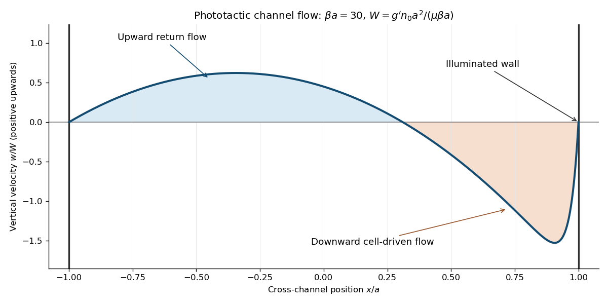
There is a genuine global qualification to the bulk construction. For an exactly steady channel with impermeable ends as well as impermeable sidewalls, the closed-channel cell-flux constraint also requires $\int J_{z}dx=0$ at every height. In this bulk ansatz the first-order orientation closure givessince integration by parts, $n^{\prime }=\beta n$ and $w(\pm a)=0$ imply $\int n{w}^{\prime }=-\beta \int nw$. Moreover, multiply $\mu w^{\prime \prime }=G+g^{\prime }n$ by $w$ and integrate. The wall values and zero fluid flux givefor a nontrivial profile. Thus zero axial cell flux generally fails unless the extra factor $1+V_s\beta K_1/(2D_r)$ vanishes, or the flow is trivial. A complete steady closed-channel solution generically needs axial concentration variation. The explicit profile solves the stated bulk equations, sidewall conditions, concentration normalization and zero fluid-flux condition; it is not, for arbitrary parameters, an exact globally closed steady cell distribution. Ignoring end regions gives the intended bulk approximation, but does not by itself prove the stronger global existence claim.