Use the symmetric lossless beam splitter convention with transmission amplitude and reflection amplitude . The two mirrors contribute the same fixed quantum phase, which can be suppressed. At the rightward port , the upper-arm route has one reflection at BS1 and one transmission at BS2, while the lower-arm route has one transmission at BS1 and one reflection at BS2. Their probability amplitudes therefore add asBy the Born rule,For the upward port, the two amplitudes are and , giving and . They sum to one, as required for an ideal lossless Mach-Zehnder interferometer. Thus is bright at zero relative quantum phase and dark at quantum phase . A fixed unequal reflection quantum phase or a swapped port labeling would shift the fringe; the stated convention fixes the port and quantum phase calibration used below.
Write the unknown pure photon polarization qubit asThe polarizing beam splitter sends the component down the lower path and the component up the upper path. After rotating the upper photon polarization to , both paths have the same internal quantum state and can interfere at BS2. Absorb fixed apparatus phases into a calibrated zero for the tunable quantum phase. With the preceding reflection convention, the quantum state before BS2 is , so the two output amplitudes areConsequentlyRepeated counts while scanning determine the complex quantum coherence . The interference visibility is , and the fringe position determines the relative quantum phase whenever both components are nonzero.
A fringe alone is not enough to determine an arbitrary photon polarization quantum state: it fixes but not which of and is larger. Indeed, and both give the flat fringe . For a general pure quantum state, the two possible population differences areResolve this ambiguity by temporarily detecting the two paths before BS2. Their relative counts give and using the same polarizing beam splitter and detectors. Taking as a global-phase choice, the reconstructed quantum state for isIf , it is up to a global phase. This completes interferometric polarization tomography. The counts are obtained from many identically prepared photons; they do not identify an arbitrary quantum state from one photon.
A full fringe scan is unnecessary. Use the same components to make three fixed projective measurements, on separate batches of identically prepared photons. Direct path detection after the polarizing beam splitter measures the populations. Recombine after matching the arm photon polarizations, once with and once with , to measure the two quadratures of the quantum coherence.
In the basis, write the density matrix in terms of its Bloch vector as . The previous formula becomesThus three measured relative frequencies giveand determineThe two interferometric settings analyze the diagonal linear polarizations and the circular polarizations , with detector labels fixed by the calibrated quantum phase convention. This is informationally complete three-observable qubit tomography: direct measurements in three bases replace fitting an entire phase-dependent fringe. It also reconstructs a mixed input, for which , although the source here is assumed pure.
Simply measuring transmission through one fixed polarizing beam splitter would determine only . Rotating a linear analyzer through different angles can additionally determine , but cannot distinguish the two signs of without a relative-phase measurement. For arbitrary, possibly elliptical photon polarization, all three settings above are needed; no extra analyzer element beyond the described path-phase control and photon polarization rotator is required.
Without the upper-arm rotation, the photon polarization still labels the path. Before BS2 the quantum state isAfter the balanced beam splitter, the polarization-valued output amplitudes areThe detectors do not resolve photon polarization. Since , the cross terms vanish in the Born rule:These probabilities are independent of the tunable quantum phase and the input photon polarization, so there is no usable wave interference fringe. Equivalently, taking the partial trace over photon polarization removes the quantum coherence between the two path quantum states. The which-path information is retained in orthogonal photon polarizations even without anybody measuring it. Rotating the two occupied photon polarization quantum states to the same quantum state removes that distinction and allows the cross term in part (ii).
Put and write , with normalized. The Hadamard gates prepare the control register in . Controlled powers of the unitary operator then give quantum phase kickback:Thus the register quantum state is , while the target remains . Define the quantum Fourier transform by . Its inverse givesWhen , the inner finite geometric series equals if and zero otherwise. Therefore exact quantum phase estimation givesThe quantum phase, rather than an unrestricted integer , is recovered modulo .
The printed circuit has no bit-reversal swaps. Its top control uses , and its measured top wire gives the least significant output bit. Write . Before the top wire's final Hadamard gate, its relative quantum phase is , so that gate produces . The controlled inverse quantum phase gates then subtract its contribution from lower wires. More generally, before the final Hadamard gate on wire , the relative quantum phase isso that wire gives deterministically. For the three-wire drawing, the correct interpretation isEquivalently, its Fourier-inversion circuit is , where reverses the register bits. Relabeling the measured bits or appending swaps gives the usual integer output. This bit convention matters, for example, when quantum phase produces top-to-bottom bits , representing the label four rather than one.
Write , with . Decode the measured bits as above. The probability amplitude of label isUsing the finite geometric series,Interpret removable singularities by continuity. In particular, near-grid quantum phase estimation returns the nearby exact label with probabilityThis is near one under the stated small-offset assumption, but not exactly one when .
There is also a rigorous error bound. Taking the squared modulus of the sum giveswhere and the elementary sums of and evaluate the last expression. HenceOn that event the circular quantum phase error is at most . For other labels, the exact probabilities areTheir total is , describing the leakage from the perfect solution. The physical output bit string remains reversed in the printed circuit; this changes its decoding, not these probabilities.
A central application is quantum order finding, which supplies the quantum step in the Shor algorithm for factoring an integer . Choose an integer coprime to , and let be its multiplicative order modulo . On valid residue quantum states define the reversible modular-multiplication unitary operator , extending it reversibly to any unused computational basis quantum states.
The orbit has the orthonormal eigenstatesfor . One need not know to prepare an eigenstate: the easy input makes quantum phase estimation sample one of these eigenphases. Its control register estimates . With chosen at least of order , the nearest quantum phase label has rational approximation error small enough for continued-fraction recovery in quantum order finding. For instance, gives on the nearest-label event. If and are coprime, the recovered denominator is ; otherwise one obtains a divisor and can repeat, combine candidates and verify them by modular exponentiation.
When the verified order is even and , the greatest common divisorsgive nontrivial factors: their product is divisible by , while neither factor inside the gcd is zero modulo . Unsuccessful choices of or quantum phase samples are handled by repetition and classical verification. Controlled powers of are implemented by efficient reversible modular arithmetic, rather than by naively applying exponentially many times.
Quantum phase estimation turns modular-multiplication eigenphases into an efficiently usable period, enabling quantum factoring in time polynomial in the bit length of the integer. Factoring is important to public-key cryptography, and this is a major example of a quantum algorithm improving on known classical methods. Another use is extracting energy eigenvalues by applying quantum phase estimation to a controlled time-evolution operator, with care to avoid energy aliasing and to prepare an input having overlap with the desired eigenstate.
Number the physical wires from top to bottom and write a computational basis ket in that order. The first four are ancilla qubits and the fifth carries the input. It is enough to follow the basis input , , because the encoding quantum circuit acts linearly.
The first fan-out consists of four controlled-NOT gates from wire 5 to wires 1–4. It sends to . The three Hadamard gates then giveThe two Pauli X gates on wires 2 and 3, followed by a Controlled-Z gate and the same two X gates, restore the bits but contribute : the sign is negative exactly when the original bits on both wires were zero. Finally, the right-hand controlled-NOT gates are , , and . They leave the first three bits unchanged and turn the last two into and . ThusExplicitly, the logical basis quantum states produced by the printed gates areEach has eight orthogonal terms of equal magnitude, and their supports are disjoint, so they are normalized and mutually orthogonal. The arbitrary input is therefore encoded asThis is a realization of the five-qubit error correcting code. The input amplitudes and their relative quantum phase are preserved in the logical subspace; the encoding is an entangled-state linear isometry, not five independent copies of the unknown input. The explicit signs and bit ordering above are fixed by this circuit, rather than by a convention for a different encoder.
Assume independent physical-qubit errors with common probability , ideal encoding and recovery, and the specified rule that every block with two or more errors fails. The number of physical errors has a binomial distribution with parameters . Correct recovery occurs for zero or one error, soThe corresponding logical failure probability isAn unencoded qubit succeeds with probability . Thus encoding improves this probability precisely when . Factoring givesOn , the sign is the sign of . Its derivative is : it is positive until and negative afterwards on . Since , and its interior maximum is positive, there is exactly one zero in . The five-qubit concatenation threshold is thereforeAt the two success probabilities agree; above it this decoder makes the error rate worse. At both schemes succeed perfectly, and at both fail under the stated error model. The small- behavior exhibits cancellation of every single-qubit-error contribution.
Use a concatenated quantum error-correcting code: each of the five outer-code qubits is encoded in its own five-qubit inner block. Independent physical errors and ideal inner correction make each decoded block act as one outer qubit with error probability . Errors in distinct inner blocks remain independent in this model. Outer recovery succeeds if at most one of the five decoded blocks is bad, givingThus the two-level logical failure probability isThis improves the leading error order from for a bare qubit to for one level and for two. At least two physical errors must occur in each of two different inner blocks to defeat the prescribed two-stage decoder. Many error patterns with more than one error in the full 25-qubit register are therefore corrected: one error in each of all five blocks is removed at the inner level, and a single failed inner block is corrected at the outer level. Concentrating several physical errors in one block can be easier for this decoder than placing two errors in each of two blocks.
More generally, levels use physical qubits with recursion . For , one has . Repeated concatenation decreases to zero: its limit must be a fixed point of the continuous function , and below the only fixed point is zero. A simple quantitative bound is , obtained by the union bound over the ten pairs of possible error positions. Induction giveswhich proves rapid suppression when ; the exact threshold is the larger value . Above this recursion amplifies errors instead.
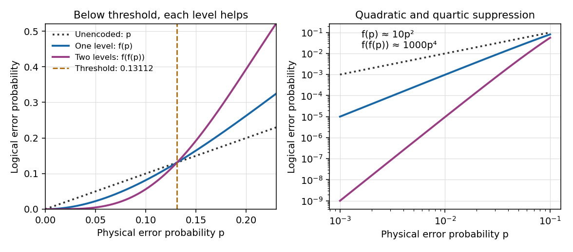
One and two levels of ideal five-qubit error correction below and above the transmission-error threshold
. Details. 
Below threshold, concatenation suppresses logical errors while allowing an entire bad inner block to be corrected at the next level. The cost is additional physical qubits, gates, syndrome extraction and recovery. The calculated threshold concerns the independent transmission-noise model with perfect encoding and recovery; including noisy operations or correlated channel errors requires a different error analysis.
For a positive operator , the spectral theorem writes with . Hence its unique positive square root of an operator is . Conjugating this spectral decomposition shows for a unitary operator .
Let and . Then and . The square-root covariance and the cyclic property of the trace giveFor the quantum fidelity, covariance first gives . ThereforeApply the same square-root identity and the cyclic property of the trace to obtainThus unitary invariance of trace distance and fidelity givesThe same acts on both quantum states: these quantities depend on the relative distinguishability of the quantum states, not on a choice of basis.
Write and . A pure-state density matrix is a rank-one orthogonal projector, so andTaking its square root and trace yields the unsquared quantum fidelityUse unitary invariance of trace distance and fidelity to choose a basis of the span of the two quantum states in which and , with and . Choosing state-vector phases to make the coefficients nonnegative does not change either density matrix. On that span,Its eigenvalues are and , with zero eigenvalues on the orthogonal complement. The positive square root of therefore has two eigenvalues , so the trace distance is . Thus the pure-state trace distance and fidelity identity isIdentical pure quantum states give ; orthogonal pure quantum states give . If the span is one-dimensional, the identical-state result follows directly, so no second basis vector is required. This formula uses the unsquared fidelity convention in the paper; if fidelity denotes squared overlap instead, the square inside the formula is omitted.
The Pauli X gate interchanges the two basis quantum states. Because the bit-flip outcome is a classical unobserved error rather than a coherent superposition, the quantum bit-flip channel givesFor , its explicit density matrix isFor a pure reference quantum state, the square of the paper's quantum fidelity is . ThereforeWith , the expectation is , the component of the Bloch vector. Hence“All possible quantum states” is interpreted as the rotationally invariant uniform pure-qubit average, with measure . Thusso the average pure-qubit fidelity of a bit-flip channel isEquivalently, rotational symmetry gives , since a pure-state Bloch vector has unit length. The eigenstates are unchanged as density matrices and have fidelity one, while a computational basis quantum state has ; these provide checks on the angular expression. A uniform distribution in rather than in solid angle would produce the wrong ensemble average. The requested quantity is the mean squared fidelity, not the square of the mean unsquared fidelity.
Articles by others on the same topic
There are currently no matching articles.