Equations and conventions. Let be a constant reference density and define total buoyancy acceleration by . With reduced pressure , the nonrotating ideal Boussinesq equations areDensity departures are small compared with , so they can be neglected in inertia and mass continuity but retained in the gravitational force. The reference stratification must also change density only weakly over the depth of interest. incompressible flow is already assumed; the Boussinesq approximation additionally restricts the size of the density variations, rather than following automatically from incompressible flow. An ideal fluid here has neither viscosity nor buoyancy diffusion.
A stationary reference profile has buoyancy frequencyStable stratification has : an upward-displaced parcel retains its old buoyancy and has negative buoyancy relative to its new surroundings.
Vorticity equation and linearization. For motion in the plane, choose the streamfunction by , . The -component of vorticity is then , where . Taking the -component of the curl of momentum givesThe minus sign in the buoyancy curl follows from .
Write with and . The linear material derivative is . The perturbation equations areThe shear-curvature term arises because advects the basic vorticity . Apply to the first equation and use the second; commutes with and does not differentiate the height-only coefficients. Therefore
For a stationary nonzero horizontal wavenumber , the buoyancy equation gives . Substitution into the vorticity equation givesHere is the Scorer parameter. Where , the vertical structure is oscillatory; where , it is evanescent. A rigid flat lower boundary gives for . In an upper evanescent region the growing solution is excluded by boundedness. When propagation persists to infinity, an appropriate radiation condition distinguishes outgoing from incoming energy for a forced problem.
If with , its curvature term vanishes. Bounded implies aloft. Thus every fixed nonzero eventually lies in an evanescent region. If stratification is sufficiently strong near the bottom, a lower oscillatory region is separated from the upper evanescent region by a turning level of a stationary internal wave. Waves reflect at that level and at the rigid lower boundary, giving vertically trapped modes for the horizontal wavenumbers that satisfy both conditions. In a slowly varying example the phase condition is approximately , from a lower node and the turning-point connection; the key point is trapping by the decrease in the Scorer parameter, not a physical lid.
Rigid channel modes. With constant and , the vertical nodes require , . Stationarity then requiresThe specified strict interval admits positive for exactly . Choosing , every real superposition of these nonzero-wavenumber modes isThe two independent complex constants encode the amplitudes and horizontal phases; negative wavenumbers are supplied by complex conjugation, not additional independent constants.
Exact finite amplitude. Put . Both modes and every superposition satisfy . For the total streamfunction , the total buoyancy is . A stationary velocity is tangent to its streamfunction contours, so exactly. Moreover the nonlinear self-advection of vanishes because it is proportional to itself. The remaining vorticity equation iswhich is an identity. Both rigid boundaries remain impermeable, and the curl-free residual in momentum determines a pressure. Thus the displayed two-mode family consists of exact finite-amplitude Boussinesq solutions, with no small-amplitude restriction on the constants in these equations. Very large amplitudes can overturn the stratification or leave the physical Boussinesq regime; exact existence does not establish stability.
The two-constant statement concerns wave disturbances with . If is literally included, arbitrary stationary horizontal shear adjustments and height-only buoyancy changes are also possible. They are changes of the basic state and are not constrained by the wave equation obtained after division by . Excluding that mean-flow sector is necessary for the intended count.
Full equations and the balanced scaling. Let , free-surface displacement and layer thickness . The inviscid rotating shallow water equations areHere gradients are horizontal and is a fixed bottom height. For horizontal scales , velocities and time scale , acceleration is , whereas the Coriolis term is . A small Rossby number therefore gives leading geostrophic balance. DefineThe last length is the Rossby deformation radius. Geostrophy gives and consequentlyThe usual distinguished quasi-geostrophic limit takes the Burger number of order one, small surface displacement, and bottom amplitude . The ageostrophic velocity is smaller than the geostrophic velocity by a factor of order , but its small divergence supplies the first nonzero thickness tendency. Motions are slow compared with , and the shallow-layer approximation also requires depth small compared with horizontal scale. Other deformation-radius limits are possible only if the small-height condition is retained.
Taking the vertical curl and combining it with thickness continuity gives exact shallow-water potential vorticity conservation,Expand to first order in relative vorticity, displacement and relief; multiplication by removes the irrelevant constant depth factor. To quasi-geostrophic accuracy,Potential-vorticity conservation transports this scalar with the geostrophic flow. Potential-vorticity inversion solves the elliptic problemwith the required boundary or far-field conditions, then differentiates to recover velocity and surface height. The deformation term suppresses the far-field influence over distances comparable with ; at scales much shorter than the inversion approaches the two-dimensional Poisson problem.
The full shallow-water system evolves two velocity components and layer thickness independently, with three first-order time equations. The quasi-geostrophic system evolves one scalar; balanced velocity and height are diagnostic consequences of inversion. In particular it filters the two fast inertia–gravity branches, whose resting-layer dispersion is , and does not describe their fast geostrophic adjustment. Reducing the time order restricts admissible initial data; it does not turn an arbitrary full shallow-water state into a quasi-geostrophic state automatically.
The intended Gaussian inversion, and its required background qualification. Set and . Direct differentiation givesConsequently, in an inversion with uniform PV and its background gradient explicitly compensated, the printed relief is balanced byThis is the Gaussian topographic response with compensated uniform potential vorticity. In that model the perturbation PV is identically zero, and any steady velocity field advects this uniform PV trivially.
There is a genuine uniform-current obstruction to constant shallow-water QG potential vorticity in the literal constant-, finite- formulation. A geostrophic background current has total streamfunction and a background free-surface slope. Over flat bottom its PV is , not uniform. For the displayed Gaussian and printed relief, the two disturbance terms cancel in inversion but leaveFor and finite this residual is nonzero; for example, it is nonzero at . Thus the claimed Gaussian is not a steady solution of the standard unforced constant- equations as literally stated. Omitting the mean contribution to the stretching term is not a legitimate gauge choice.
A precise intended repair is to supply a background PV gradient from an explicitly compensating weak bottom slope or beta-plane background, so the current really does have uniform PV. Another repair is the rigid-lid limit . In the uncompensated finite- current model, a Gaussian can instead solve steady equations if the term is removed from the relief: then and , so . Its PV is not uniform. These repairs distinguish the intended calculation from the false literal claim.
Smallness and closed streamlines of the intended response. Its maximum disturbance speed isIts relative vorticity is of order , and its surface displacement has maximum . The relief satisfies . Sufficient conditions for quasi-geostrophic consistency are thereforeThe second condition limits the background geostrophic height change across the disturbance scale. The last controls disturbance Rossby number, surface height and bottom relief, including positive layer depth. For comparable with it reduces to . It does not require disturbance velocity to be small relative to .
Take without loss of horizontal orientation. The total streamfunction is , withIf , then everywhere and no streamline can close. In terms of the relief amplitude,is the strict no-closed-cell condition. Above this closed-streamline threshold for a Gaussian disturbance in uniform flow, stagnation points occur at on the side opposing the current. The equation has two roots: the inner one is a center because both Hessian eigenvalues of have the same sign; the outer one is a saddle. Closed contours surround the center and are bounded by a separatrix. Equality gives a degenerate onset, with no finite-area closed cell yet. If , every nontrivial Gaussian response instead has circular closed streamlines.
Closed streamlines are compatible with small Rossby number: their threshold can be reached with of order the already small background Rossby number. They do not alone invalidate quasi-geostrophy. They do, however, disconnect the cell from upstream PV data. If only the upstream PV is specified, the PV in such a cell depends on its formation history and cannot generally be assigned from the upstream value alone. Globally uniform initial PV would remain uniform in the ideal compensated model, but mixing, dissipation and forcing history can select a different physical trapped circulation. These qualifications are separate from the constant- inconsistency demonstrated above.
Balanced variables and PV derivation. Write the disturbance reduced pressure as . Leading geostrophic balance gives , and leading hydrostatic balance gives buoyancy anomaly . The geostrophic material derivative isIt includes horizontal advection, not an independent prognostic vertical velocity. The appropriate regime has small Rossby number, small stratified Froude number, thin aspect ratio and slow evolution; a common scaling has of order one and .
Only the vertical rotation component is retained in the traditional approximation. In the horizontal momentum balance, the horizontal part of the rotation vector multiplies the small vertical velocity; in vertical momentum, its contribution is small compared with leading hydrostatic pressure and buoyancy in the thin-layer scaling. Away from the equator these corrections are smaller by a factor of order . They need not be small in equatorial or strongly nonhydrostatic settings, so the approximation has a definite regime of validity.
Put . Eliminating from buoyancy givesThe last step needs justification because and do not commute on arbitrary fields. Their extra terms here areSubstitution into the supplied vorticity equation givesSince ,This is three-dimensional quasi-geostrophic potential vorticity conservation; the height-dependent coefficient is retained inside the derivative.
At a small steady lower elevation , impermeability gives , evaluated at to leading order. Substitution into buoyancy and division by gives the topographic buoyancy boundary condition for quasi-geostrophic flow,
Rossby waves at rest. For constant let and . Linearization about relative rest gives . A Fourier wave givesFor , the zonal phase speed is westward. At fixed altitude the PV perturbation is ; its total field is the background with sinusoidally displaced contours, as sketched below.
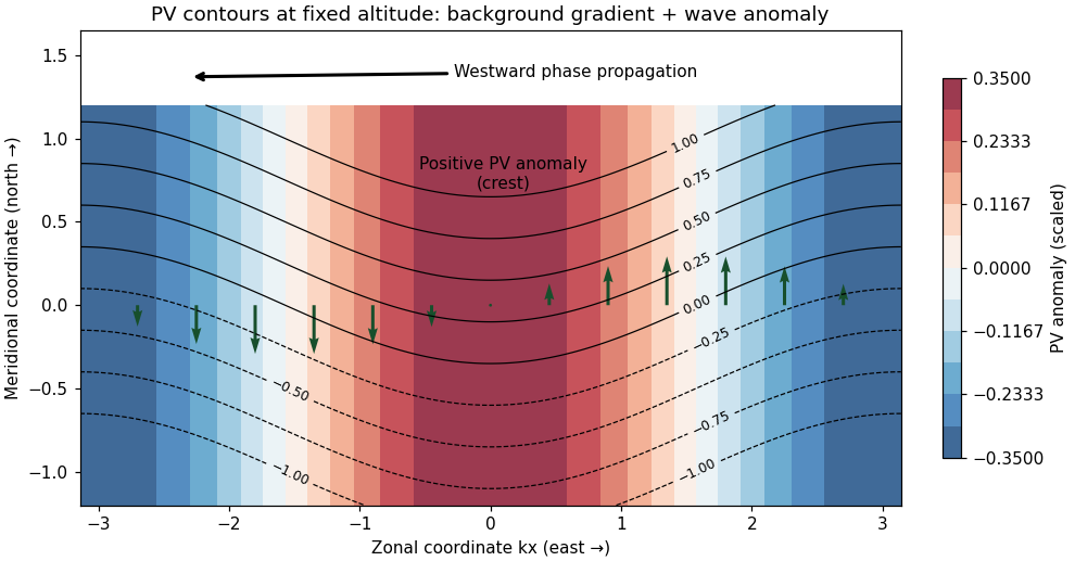
Rossby-wave PV contours and meridional flow producing westward phase propagation
. Details. 
A northward parcel displacement has : it retains the smaller background PV of its origin. The inverted geostrophic velocity associated with a positive PV crest is northward on its eastern flank and southward on its western flank. Advection of the background PV then decreases the anomaly on the eastern flank and increases it on the western flank, shifting the crest westward. This is a PV-restoring mechanism, not a westward mean current.
Differentiating the dispersion relation gives the group velocityFor nonzero , the vertical phase speed is , soThus upward energy propagation accompanies downward vertical phase propagation, and conversely. For the vertical group speed is zero and a vertical phase speed is not defined.
Stationary topographic response. Assume , and nonzero corrugation wavenumber . In a uniform current the laboratory dispersion is . For a stationary quasi-geostrophic mountain wave, , givingFor , the linear lower-boundary condition becomes . Its forced nonzero- component therefore hasIf , the vertical wavenumber is real. Both signs would be bounded aloft, so boundedness alone is insufficient for uniqueness. Impose an upward radiation condition, excluding waves incident from infinity; equivalently switch on the terrain forcing causally with arbitrarily weak absorption aloft. Since has the sign of , chooseThe unique outgoing forced component is thenThe bottom derivative and verify the phase and amplitude. In this stationary pattern it is the intrinsic frequency that describes downward vertical phase propagation relative to the current; the laboratory frequency is zero.
If or , defineExclude exponential growth at infinity. The unique decaying forced component isAt the excluded value , a nonzero prescribed bottom derivative cannot be matched by a bounded constant/linear vertical solution; the steady idealization is singular. At the boundary is not crossed and there is no forced response in the linear nonzero- sector: , rather than an expression obtained by dividing by . Uniqueness throughout refers to the prescribed forced Fourier component, with the reference state fixed and no independently incident waves or added mean-state changes.
The propagation criterion explains why topographically forced planetary Rossby waves can carry energy into a moderately westerly stratosphere, while easterlies and sufficiently strong westerlies block their vertical propagation. Larger horizontal scales more readily meet the criterion. Real dissipation, height-dependent winds and critical levels modify the simple solution and allow wave–mean-flow interaction; the ideal constant-coefficient calculation establishes the propagation filter, not a complete theory of stratospheric evolution.
Stable stratification is a constraint on motion, not an isolated parcel spring. A light-over-heavy density profile has . An adiabatically displaced parcel has buoyancy anomaly relative to its surroundings. If one neglects the pressure response and movement of surrounding fluid, the vertical equation would be . A finite spherical blob cannot satisfy that isolated-oscillator picture: incompressible flow requires surrounding fluid motion, and the pressure perturbation communicates its acceleration to the rest of the fluid.
This can be shown directly with the linear Boussinesq equations. For a uniform background, take a Fourier wavevector . Pressure removes the component of the buoyancy force parallel to this wavevector. Taking the divergence of momentum to determine pressure and projecting the vertical component givessoThis pressure projection in a displaced stratified blob produces frequencies less than except for wavevectors with . A localized spherical perturbation contains a range of directions and therefore a range of frequencies. It deforms and emits internal gravity waves, rather than remaining one sphere oscillating coherently at . The added mass of a rigid sphere is a useful inertia analogy, but its numerical correction does not define an exact oscillation frequency for a deformable material blob in stratified fluid.
Internal waves and energy transport. The restoring force supports anisotropic internal gravity waves: their frequency depends on the direction, not just the length, of the wavevector. For a two-dimensional positive-frequency branch, with . Differentiation givesThe vertical group and phase velocities have opposite signs. Wave energy therefore travels along a direction different from the direction of phase propagation, a point essential in selecting radiation conditions for wave-generating obstacles.
For constant , the linear perturbation energy density per reference mass isDot momentum with velocity and multiply buoyancy evolution by ; the terms cancel, leaving . The second term is the available potential energy stored by displacement against the stable density profile. In an ideal fluid, that energy is exchanged with kinetic energy or transported away, not irreversibly dissipated by buoyancy diffusion.
Steady flows, layers and topography. Stable stratification penalizes vertical displacement and favors flows with small vertical motion when the stratified Froude number is small. The natural vertical displacement scale associated with kinetic energy is of order ; obstacles requiring much larger displacements can cause blocking and diversion instead of simple overpassing. In the ideal model fluid retains its buoyancy label, so motion tends to follow density surfaces. This inhibits vertical mixing but does not forbid horizontal rearrangement or turbulence powered by a shear flow.
A uniform current crossing topography generates stationary internal waves when its intrinsic frequency lies in the internal-wave range. For horizontal wavenumber , stationarity gives . Height-dependent wind and stratification replace this by the Scorer parameter relation derived in Question 1. A decrease of that parameter can produce a turning level, evanescence and vertical trapping, explaining lee-wave trains confined near a lower boundary. The exact channel superpositions in Question 1 also show that nonlinearity does not automatically destroy every wave solution.
Stability of the background density profile does not imply stability of every flow built on it. Sufficiently large waves can overturn density surfaces, and shear can supply energy to disturbances. Ideal advection can create fine structure, but irreversible homogenization of buoyancy in a real fluid additionally involves diffusion or dissipation. A finite-amplitude ideal solution is consequently distinct from a guaranteed stable or physically realizable state.
How rotation changes the picture. With the vertical Coriolis parameter , the corresponding uniform-background inertia–gravity dispersion becomesWhen , the propagating branch lies between and . Rotation also allows a slow balanced sector: horizontal pressure and Coriolis forces balance, vertical pressure and buoyancy balance, and the circulation can be described through potential-vorticity inversion. Small Rossby number and small stratified Froude number lead to the quasi-geostrophic equations rather than to the fast internal-wave dynamics. Vertical shear is then tied to horizontal buoyancy gradients through thermal-wind balance.
In this balanced sector, a planetary or topographic PV gradient supports Rossby waves, whose restoring mechanism is conservation of PV under displacement across that gradient. Stable stratification couples horizontal levels through the term, and the mountain-wave calculation in Question 3 illustrates its vertical propagation filter. Thus stratification can support rapid buoyancy-restored waves, constrain slowly evolving balanced circulation, and shape interactions with boundaries; which description applies depends on the velocity, length, time and rotation scales.
Articles by others on the same topic
There are currently no matching articles.