Past exam of the mathematics course of the University of Cambridge / 2006 / iii / Paper 38 (Mathematics of Operational Research)

Introduce slack variables $s_1,s_2,s_3$. The initial simplex dictionary isAll six variables are nonnegative. The given rule is the Dantzig pivot rule: select the nonbasic variable with the largest positive reduced cost. It applies to slack variables too once they become nonbasic. At each step the simplex ratio test limits how far that entering variable can increase before a basic variable reaches zero.

The successive objective rows of the simplex dictionary, expressed in the current nonbasic variables, areThese rows identify each entering variable unambiguously. Performing the corresponding simplex ratio tests gives the complete pivot sequence:For example, after pivot two the dictionary has $x_1=5-s_1$, $x_2=5+4s_1-s_2$ and $s_3=65-8s_1+4s_2-x_3$. Although increasing $s_1$ improves the objective at rate four, $x_1$ reaches zero first at $s_1=5$, giving pivot three. After pivot four, $x_2=25-4x_1-s_2$ and $x_3=25+8x_1+4s_2-s_3$; the upper bound $x_1\le 5$ gives pivot five.

In the final objective row every reduced cost is nonpositive. Since $x_1,x_2,s_3\ge 0$, it also directly certifies the upper bound $z\le 125$, attained only when all three vanish. Thus

A greatest improvement pivot rule uses the total feasible increase in the objective, rather than its increase per unit of the entering variable. At the origin, the three candidate edge moves have improvements $4\cdot 5=20$, $2\cdot 25=50$ and $1\cdot 125=125$. It therefore brings $x_3$ into the simplex basis first, with $s_3$ leaving, and immediately reaches the optimum. This rule solves this instance in one pivot.

This is a three-dimensional Klee-Minty cube example: the specified Dantzig pivot rule visits every vertex before reaching the optimum. Higher-dimensional versions require $2^d-1$ pivots, so that rule has exponential worst-case running time despite its strong practical performance. Each pivot requires only polynomially many arithmetic operations. An anti-cycling rule such as the Bland pivoting rule ensures finite termination; without one, degenerate pivots can cycle. A crude terminating bound is the number of possible bases, $\left(\genfrac{}{}{0ex}{}{m+n}{m}\right)$ for $m$ constraints and $n$ original variables, which can be exponential. This does not show that every conceivable pivot rule must take exponential time. Linear programming itself has polynomial-time algorithms, including the ellipsoid method and suitable interior-point methods.

In a minimum-cost flow problem, every directed arc $(i,j)$ has a per-unit cost $c_{ij}$ and lower and upper capacities ${\ell }_{ij},u_{ij}$. Each vertex has a prescribed net supply $b_i$, with ${\sum }_i{b}_i=0$. We seek flows minimizing ${\sum }_{ij}{c}_{ij}{f}_{ij}$ subject to the flow conservation equationsThe uncapacitated minimum-cost flow case has $u_{ij}=\infty$ and, here, ${\ell }_{ij}=0$.

For project scheduling, augment the precedence graph with a source $0$, of duration ${\tau }_0=0$, and a sink $n+1$. Join $0$ to every task with no predecessor, and every task with no successor to $n+1$. Extend the precedence matrix to these dummy arcs. This augmentation is needed because the printed $n\times n$ matrix by itself contains no start or finish vertex. Assuming the precedence graph is a Directed acyclic graph, every task lies on a source-to-sink path. Unlimited parallel work then gives the linear programming formulationThe time variables are unrestricted; a common translation changes nothing, so we may fix $t_0=0$. These inequalities say that each successor starts after its predecessor finishes. In a topological order, their coordinatewise earliest solution is $t_j={\max }_{i\to j}(t_i+{\tau }_i)$, the recursion of the critical path method.

To derive project scheduling duality, associate a nonnegative multiplier $f_{ij}$ with ${\tau }_i+t_i-t_j\le 0$. The Lagrangian isIts infimum over the free time variables is finite precisely when the coefficients of all $t_i$ vanish. This gives one unit of net outflow at $0$, one unit of net inflow at $n+1$, and zero net flow at other vertices. Hence the dual isEquivalently, minimize $\sum c_{ij}{f}_{ij}$ with $c_{ij}=-{\tau }_i$. The project duration is the negative of the optimal minimum-cost flow value. The sign is essential: the dual of the minimization problem maximizes total duration, selecting a longest precedence path.

The network simplex algorithm is a general method for minimum-cost flow. After shifting lower bounds to zero, first find a feasible flow, using artificial arcs and a phase-one objective if needed. A network simplex tree basis fixes each non-tree arc at a bound and determines the tree flows by flow conservation. Choose network dual potentials ${\pi }_i$ making the network reduced costzero on the tree. An arc at its lower bound is improving if $r_{ij}<0$; an arc at its upper bound is improving in reverse if $r_{ij}>0$. Adding that residual arc creates one fundamental cycle. Increase flow around this cycle until an arc reaches a bound, then exchange the entering and leaving tree arcs, or flip the entering arc to its other bound. The flow conservation equations remain satisfied. Use an anti-cycling rule for degenerate pivots. If a negative-cost residual cycle has no finite limiting capacity, the objective is unbounded below; if phase one cannot remove artificial flow, the problem is infeasible. Otherwise, termination with no negative residual network reduced costs certifies optimality, since potentials cancel around cycles and every residual network circulation has nonnegative cost.

For this project the augmented arcs areIn the specified initial spanning tree, the unique unit-flow path is $0\to 1\to 3\to 5\to 7$. The flow on its arcs is one and that on all other tree arcs is zero. Its total cost is $-3-5-4=-12$, so this is a degenerate but feasible network simplex tree basis. Normalizing ${\pi }_0=0$, the tree equations giveThere are two nonbasic arcs. Their network reduced costs areBring $(0,2)$ into the tree. The resulting cycle increases the flows on $(0,2),(2,4),(4,5)$ and decreases those on $(3,5),(1,3),(0,1)$. The three decreasing arcs initially carry one unit, so the maximal step is one. Resolve the leaving-arc tie by removing $(0,1)$. The resulting unit flow follows $0\to 2\to 4\to 5\to 7$ and has cost $-4-6-4=-14$.

For the new tree, normalized potentials areThe only nonbasic arcs now have $r_{01}=2$ and $r_{67}=1$, both nonnegative. All tree network reduced costs vanish, proving optimality after this single pivot. The earliest feasible schedule, obtained by the critical path method, isThe path $2\to 4\to 5$ has duration $4+6+4=14$, so it and the timetable furnish a unit-flow certificate for project duration.

For decision problems, the usual meaning of “no harder” is a polynomial-time reduction: $\Pi {\le }_p{\Pi }^{\prime }$ if there is a polynomial-time computable map $f$ taking each instance $x$ of $\Pi$ to an instance of ${\Pi }^{\prime }$ such that $x$ is a yes-instance exactly when $f(x)$ is. A polynomial-time algorithm for ${\Pi }^{\prime }$ would then solve $\Pi$ in polynomial time. A problem is NP-hard if every problem in NP admits such a reduction to it.

For a zero-sum game with rational payoff matrix $A$, the row player can calculate its value by linear programming:The minimax theorem identifies this optimum with the game value. Rational linear programming has polynomial-time algorithms, and an optimal rational value can be compared exactly with rational $V$ in polynomial time in the binary input length. Thus the decision problem belongs to P. If it were NP-hard, composing the reductions with this algorithm would put every problem in NP in P, contradicting the assumed separation. ThereforeThe finite rational encoding is part of the computational model; arbitrary real inputs without an encoding would not define the same complexity question.

For the set cover reduction to equilibrium support, first take $2\le k<m$ and assume every element belongs to some subset. Suppose rows $i_1,\dots ,i_k$ cover $S$. Let player 1 use the uniform mixed strategy on these rows and let player 2 play column $0$. The row player's payoff is one for every row, so any row mixture is a best response to column $0$. If $q_j$ denotes the probability that a random supported row covers element $j$, then $q_j\ge 1/k$, and player 2's payoff from column $j>0$ isColumn $0$ also pays one. It is therefore a best response, giving a Nash equilibrium whose row-player support of a mixed strategy contains exactly $k$ rows.

Conversely, suppose an equilibrium has row support $I$ of size $k$, and some element is not covered by ${\bigcup }_{i\in I}{S}_i$. For that column $q_j=0$, so player 2 can earn $k/(k-1)>1$. This is the largest possible column payoff, and it is attained exactly at columns corresponding to elements uncovered by $I$. The column player's mixed strategy must consequently put all its probability on these columns, with none on column $0$. Every currently supported row gives player 1 payoff zero. Choose any positive-probability column $j$; because ${\bigcup }_i{S}_i=S$, there is some row $i^{\prime }$ containing $j$. Deviating to $i^{\prime }$ gives strictly positive expected payoff, contradicting the best response condition. Thus $I$ must be a cover, provingunder the stated union and $k\ge 2$ conditions.

The printed formulation omits both conditions. For $k=1$, its payoffs contain division by zero. Without the union condition its claimed implication is false: take $n=2$, $m=3$, $k=2$ and $S_1=S_2=S_3=\{1\}$. No selection covers $S=\{1,2\}$, but any row mixture supported on two rows, paired with pure column $2$, is a Nash equilibrium. The row player always gets zero, and column $2$ is the column player's strictly optimal choice with payoff two. This gives an explicit counterexample to the unrestricted wording.

These restrictions do not weaken the complexity conclusion. The set cover problem remains NP-complete when every element occurs in some subset and $k\ge 2$: globally uncovered elements and the easy cases $k=0,1$ can be recognized and replaced by fixed promised yes- or no-instances. A cover by at most $k<m$ subsets can be padded to exactly $k$. The constructed game has polynomial size, so deciding whether a Nash equilibrium of the specified support size exists is NP-hard. Computing a complete description of all equilibria would resolve this question and hence is at least this difficult. In addition, the equilibrium set may be infinite; a complete output must then describe families rather than list individual points. There is a finite representation by feasible pairs of supports and their associated strategy polytopes, but there are exponentially many support pairs to consider. This reduction concerns locating specified supports or describing all equilibria, rather than finding one unrestricted equilibrium.

The SIPV model concerns a fixed number of bidders competing for one object. Each bidder knows their own private valuation; the value of winning depends on that valuation alone. Valuations are independent random variables with the same atomless distribution $F$, known to everyone, and bidders have identical roles and access to the same strategies. The standard revenue equivalence setting also assumes risk neutrality, quasilinear utility, and noncooperative bidding: expected utility is valuation times winning probability minus expected payment.

The revenue equivalence theorem states that auctions with the same equilibrium allocation probability $p(v)$ for each type and the same expected utility for the lowest type have the same expected payment by each type, and therefore the same expected seller revenue. In particular, if the object goes to the highest valuation and the lowest type has zero expected utility, then all such auctions have the same expected revenue. In a strictly increasing symmetric equilibrium, $p(v)=F(v{)}^{n-1}$.

For a bidder of valuation $v$, the profit as a function of winning probability is $vp-e(p)$. At an interior stationary point $p(v)$,The chain rule then gives the first two identities:Integrating from zero and using integration by parts gives the interim payment identityWith the usual zero-payment normalization $e(p(0))=0$, this becomesStationarity alone does not determine the integration constant: a fixed participation fee would add that constant. The stated formula uses the lowest-type normalization from revenue equivalence.

For the lowest-price auction with independent uniform distributions on $[0,1]$, consider the symmetric increasing equilibrium, so that $p(v)=v^{n-1}$. The zero type can bid zero, lose almost surely, and pay nothing. The interim payment identity therefore yieldsSum this expected payment over the $n$ bidders and average over their uniform distributions:This uses $n\ge 2$, as appropriate for this auction format.

For three bidders, assume the common bid is $Av$ with $A>0$. If a bidder deviates to $Az$, $0\le z\le 1$, they win precisely when both opposing valuations $u,w$ are below $z$. On that event they pay $A\min (u,w)$, so their expected payment and profit areFor $0<v<1$, stationarity at $z=v$ gives $2v^2-A{v}^2=0$, henceThis is a global best response, not merely a stationary point: for $A=2$, $\partial U/\partial z=2z(v-z)$ is positive for $0<z<v$ and negative for $v<z\le 1$. Any bid above $2$ gives the same sure-win payment as $z=1$ and cannot improve the payoff.

The uniform lowest-price auction equilibrium also verifies the revenue calculation constructively for any $n\ge 2$. If opponents bid $(n-1)u$, a deviation to $(n-1)z$ has profitThus $z=v$ is optimal and $b(v)=(n-1)v$ is a symmetric Bayesian Nash equilibrium. The realized price is $(n-1)$ times the minimum valuation; this order statistic has expectation ${\int }_0^1(1-t{)}^{n}dt=1/(n+1)$, giving the same expected revenue.

A Nash equilibrium of a multi-person game is a collection of strategies such that each player's strategy is a best response to the others: no unilateral change raises that player's expected payoff. For mixed strategies, every pure action used with positive probability must attain the same maximal payoff. Take $c>0$.

In this costly turnout game, compute the payoff difference between voting and abstaining, holding the others' strategies fixed. The opponent $A$ is pivotal exactly when one of $B,C$ votes. Without $A$ the proposition then passes, while with $A$ the tied ballot fails. The pivotal voting probability is $2\beta (1-\beta )$, soIf $A$ mixes with $0<\alpha <1$, indifference is necessary. Therefore

For supporter $B$, voting is pivotal when $A$ abstains and $C$ abstains, or when $A$ votes and $C$ votes. Thus its voting advantage, and likewise that of $C$, isAt $(\alpha ,\beta )=(1,3/4)$, this equals zero, while ${\Delta }_A=c(16(3/4)(1/4)-3)=0$. Every player is indifferent between voting and abstaining at these opponent strategies; in particular, $A$'s pure vote and both supporters' mixtures are best responses. Hence

It is not unique. At $(\alpha ,\beta )=(0,1/4)$, both supporter advantages are $4c(3/4)-3c=0$, and ${\Delta }_A=0$ again. This gives a second symmetric Nash equilibrium. To see these are the only equilibria with a common supporter probability, note that $\beta =0$ or $1$ makes ${\Delta }_A=-3c$, forcing $\alpha =0$; neither endpoint then satisfies the supporters' best response condition. For $0<\beta <1$, supporter indifference requiresIf $A$ also mixes, its two possible values $\beta =1/4,3/4$ force $\alpha =0,1$ respectively, contradicting strict mixing. Finally $\alpha =0$ gives $\beta =1/4$, and $\alpha =1$ gives $\beta =3/4$. Thus

Allowing $B,C$ to have distinct probabilities $\beta ,\gamma$ gives two additional Nash equilibria. The three voting advantages areIf both supporters mix, subtracting their indifference equations gives $(2\alpha -1)(\gamma -\beta )=0$. At $\alpha =1/2$ a supporter has advantage $-c$, so cannot mix; hence $\beta =\gamma$ and the two symmetric equilibria result. If $B$ always abstains and $C$ mixes, the latter's indifference gives $\alpha =1/4$, and $A$'s indifference gives $\gamma =3/8$. Then ${\Delta }_B=-3c/4<0$, so abstention really is optimal. Interchanging $B,C$ gives the other equilibrium. If $B$ always votes and $C$ mixes, the corresponding equations give $\alpha =3/4$, $\gamma =5/8$, but ${\Delta }_B=-3c/4$, contradicting voting. The four configurations with both supporters pure also fail a best response condition. Consequently the full collection of turnout equilibria with two supporters and one opponent is

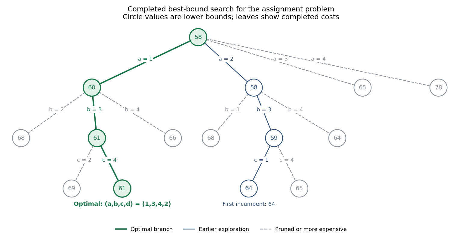
A branch and bound algorithm partitions the feasible set into subproblems and attaches a valid lower bound to each subproblem's possible objective value. A completed feasible solution supplies an incumbent upper bound. For minimization, discard a node if it is infeasible or its lower bound is at least the incumbent; otherwise branch by fixing an additional decision. The best-bound search rule expands the active node with the smallest lower bound. Once every active bound is at least the incumbent, the incumbent is optimal.

For this assignment problem, use the assignment lower bound from independent task minima. For a partial assignment $P$, with unassigned machines $M$ and unassigned tasks $J$, it isThis may reuse the same machine in several minima. Relaxing the distinct-machine constraint only reduces the cost, so the resulting lower bound is valid.

The given tree has already expanded the $a=2$ node of bound $58$, then its $b=3$ child of bound $59$. That child completes to $(a,b,c,d)=(2,3,1,4)$ at cost $12+13+11+28=64$, or $(2,3,4,1)$ at cost $12+13+23+17=65$. Thus we have an incumbent $64$. The best remaining active node is $a=1$, with lower bound $60$. Its three branches have boundsThe first and third children cannot improve the incumbent. Expand $a=1,b=3$, the sole active bound below $64$. Its last two possible completions areUpdate the incumbent to $61$. The unexpanded nodes have bounds $64,65,66,68,68,78$, all at least $61$; the other completed leaves are also more expensive. The branch and bound search therefore terminates, withThe additional expansion order after the supplied tree is $a=1$, then $a=1,b=3$. The feasible assignment of cost $61$ and the bounds excluding every remaining branch together certify global optimality.