Past exam of the mathematics course of the University of Cambridge / 2007 / iii / Paper 67 (Physical Cosmology)

A comoving coordinate labels a position relative to the homogeneous expansion. For two nearby comoving positions separated by $\Delta \chi$, their proper distance in cosmology at time $t$ is $a(t)\Delta \chi$. Thus a fixed comoving separation expands physically with the scale factor, while a fixed proper separation corresponds to a shrinking comoving separation. Normalize $a_0=1$, so $a(z)=1/(1+z)$.

At a common cosmological redshift, a transverse proper size $l$ subtends $\theta \simeq l/D_A$, where $D_A$ is the angular diameter distance. At $z=3$, a $5$ comoving Mpc separation has proper size $5/(1+3)=1.25$ Mpc. HenceThe proper-size object has the larger angular size, by a factor of four. This comparison does not require a numerical angular diameter distance, since it cancels.

Pressureless matter obeys the cosmological perfect-fluid continuity equation, ${\dot{\rho }}_m+3H{\rho }_m=0$. Integrating gives ${\rho }_m={\rho }_{m,0}(a_0/a{)}^3$. Define the present critical density and cosmological density parameters byHere $c=1$ and the curvature contribution is an effective density parameter, not an additional matter fluid. Substitution into the Friedmann equation givesUsing the Hubble parameter $H=\dot{a}/a$ therefore yieldsAt $a=a_0$ the same equation implies ${\Omega }_{m,0}+{\Omega }_{k,0}+{\Omega }_{\Lambda ,0}=1$. The power in the matter term is $a_0^3$; the converted TeX's $a_0^2$ is an error not present in the original PDF.

On an expanding branch with $\dot{a}>0$, minimizing $\dot{a}$ is equivalent to minimizing its square. Differentiating the preceding Friedmann equation with respect to $a$ givesFor positive matter density and a positive cosmological constant, it vanishes uniquely atThe second derivative is $H_0^2[2{\Omega }_{m,0}{a}_0^3/a^3+2{\Omega }_{\Lambda ,0}]>0$. Thus this is the minimum expansion speed in a matter-Lambda universe. The matter and vacuum densities satisfy ${\rho }_m=2{\rho }_{\Lambda }$ there, precisely the transition from deceleration to acceleration in the Friedmann acceleration equation.

The conclusion concerns an expanding branch that actually reaches this value of $a$. A sufficiently closed model can recollapse before reaching it; positive $\Lambda$ alone does not rule that out. In flat or open models with the stated positive densities the minimum is reached. The degenerate zero-speed limiting case requires separate treatment and does not describe a finite-time passage through a positive-speed minimum.

The stationary-point relation is ${\Omega }_{m,0}{a}_0^3/a_{\min }=2{\Omega }_{\Lambda ,0}{a}_{\min }^2$. ConsequentlyTaking the positive root on the expanding branch and eliminating $a_0$ with the result of part (iii),The bracket must be positive for a genuine passage through this minimum expansion speed in a matter-Lambda universe. Negative values mean that this formal value of the scale factor is not accessible on the corresponding physical expanding solution.

For a spatially flat model, ${\Omega }_{k,0}=0$, so ${\dot{a}}_{\min }^2/a_{\min }^2=3H_0^2{\Omega }_{\Lambda ,0}$. With the squared definition of $E$ used in the paper,Equivalently $1+z_{\min }=a_0/a_{\min }=(2{\Omega }_{\Lambda ,0}/{\Omega }_{m,0}{)}^{1/3}$, and substitution into $H^2/H_0^2={\Omega }_{m,0}(1+z{)}^3+{\Omega }_{\Lambda ,0}$ gives the same answer. The minimum is in $\dot{a}$, not in the Hubble parameter $H$, which continues to decrease towards $H_0\sqrt{{\Omega }_{\Lambda ,0}}$.

In a spatially flat FLRW metric, a radial null geodesic satisfies $d\chi =cdt/a(t)$. Normalize $a_0=1$. The comoving particle horizon at time $t$ is therefore $r_h=c{\int }_0^{t}d{t}^{\prime }/a(t^{\prime })$, using the initial singularity as the time origin. The cosmological redshift relation $1+z=1/a$ givesFor matter and a cosmological constant in a spatially flat model, the Friedmann equation gives $H(z)=H_0[{\Omega }_{m,0}(1+z{)}^3+{\Omega }_{\Lambda ,0}{]}^{1/2}$. The initial singularity corresponds to $z\to \infty$, so reversing the integration limits yieldsThis is a comoving particle horizon, not a distance to the source currently observed at redshift $z$, and not a future-directed cosmological event horizon. The corresponding proper horizon radius at that epoch is $r_h(z)/(1+z)$.

For an Einstein-de Sitter universe, the Hubble parameter is $H(z)=H_0(1+z{)}^{3/2}$. The comoving particle horizon becomesThusIt tends to zero towards the initial singularity and increases without bound as $z\to -1$ in the infinite future. At the present time it is $2c/H_0=3c{t}_0$, since the Einstein-de Sitter universe has age $t_0=2/(3H_0)$.

Use the stipulated common normalization $A=H_0{\Omega }_{m,0}$ and plot $R=A{r}_h/c$. The Einstein-de Sitter universe has $H_{0,E}=A$, whereas the $({\Omega }_{m,0},{\Omega }_{\Lambda ,0})=(0.3,0.7)$ model has $H_{0,\Lambda }=A/0.3$. Their comoving particle horizons are thereforeBoth decrease with increasing $z$, or increase with cosmic time. The Einstein-de Sitter universe curve diverges at $z=-1$ and has $R_E(0)=2$, $R_E(2)=2/\sqrt{3}$. The matter-plus-vacuum curve remains finite at $z=-1$: the integrand approaches a constant there, and its high-redshift tail is integrable. Moreover it lies below the Einstein-de Sitter curve for this particular normalization, since, with $u=1+z^{\prime }>0$,The high-redshift ratio of the two curves tends to $\sqrt{0.3}$, not one. Holding $H_0\sqrt{{\Omega }_{m,0}}$ fixed would give a different comparison; it is $H_0{\Omega }_{m,0}$ that the original question specifies.

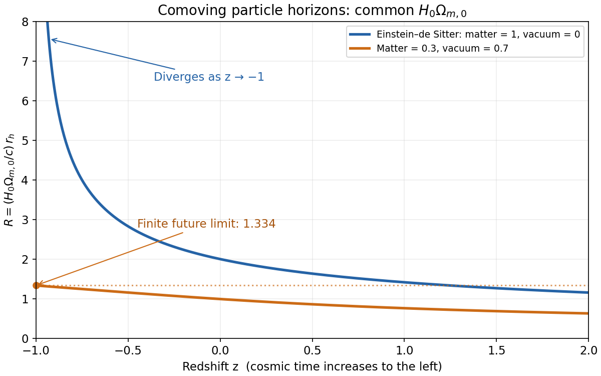
A positive cosmological constant eventually makes the scale factor grow exponentially. The future integral ${\int }_t^{\infty }cd{t}^{\prime }/a(t^{\prime })$ then converges, so the remaining conformal time is finite. The comoving particle horizon approaches a finite limiting visibility radius; it does not shrink. The remaining distance to that limit is the comoving radius of the cosmological event horizon. Thus a signal emitted sufficiently far away today can never reach us, even though the proper particle-horizon radius continues to grow. This is the total conformal lifetime of a flat matter-Lambda universe.

Normalize the Einstein-de Sitter universe by $a(t_0)=1$, giving $a(t)=(t/t_0{)}^{2/3}$. A photon emitted inward today at the current comoving particle horizon starts at ${\chi }_0=3c{t}_0$. By time $t$ it has traversed the comoving distanceAt arrival at Earth this equals ${\chi }_0$, hence $(t/t_0{)}^{1/3}=2$ andThe emitting point is at the horizon location today, not a photon already arriving today from the initial singularity. The calculation of photon arrival from an Einstein-de Sitter particle horizon follows the future inward null geodesic from that event.

For a radial null geodesic in a spatially flat universe, the comoving radial distance increment is $d\chi =cdz/H(z)$. If the cloud and quasar redshifts differ only slightly, take $H$ at their common approximate epoch $z_{\ast }$, givingMultiplying by the scale factor at that epoch gives the local proper distance in cosmology relevant to the quasar's radiation flux:If distance is instead expressed in comoving units, it is $(1+z_{\ast })d_{cq}$. Equivalently the small rest-frame velocity difference is $\delta v=c\delta z/(1+z_{\ast })$, and $d_{cq}\simeq \delta v/H(z_{\ast })$. This quasar-cloud redshift separation assumes the redshift difference is due to homogeneous expansion, with negligible peculiar velocities. Since the two observations lie on a light cone, the proper separation is understood as the short separation on a nearly common cosmic-time slice; specifying the epoch matters at higher order.

In an Einstein-de Sitter universe, $H(z)=100h(1+z{)}^{3/2}\mathrm{km}{\mathrm{s}}^{-1}\mathrm{Mp}{\mathrm{c}}^{-1}$. At the cloud's approximate epoch $z_{\ast }=3$, $H=800h\mathrm{km}{\mathrm{s}}^{-1}\mathrm{Mp}{\mathrm{c}}^{-1}$, and $\delta z=0.1$ corresponds to $\delta v\simeq 7500\mathrm{km}{\mathrm{s}}^{-1}$. ThereforeChoosing the midpoint $z_{\ast }=3.05$ instead gives $9.1h^{-1}\mathrm{Mpc}$ proper. Thus the intended approximate proper distance is about $9h^{-1}\mathrm{Mpc}$; the small variation reflects the epoch choice in the local expansion, not a factor-of-four physical discrepancy. For example the exact comoving separation is $2c{H}_0^{-1}[(1+z_c{)}^{-1/2}-(1+z_q{)}^{-1/2}]$, whose conversion at the midpoint agrees with that estimate.

At the same accuracy as the small-separation conversion, its coefficient is fixed at the cloud's well-determined epoch. Since $d_{cq}$ is proportional to $\delta z=z_q-z_c$ and $\Delta z_c$ is negligible,The given emission-redshift error corresponds near $z=3$ to $\Delta z_q\simeq (1+z)1000/c\simeq 0.0133$. HenceThe uncertainty is about $1.2h^{-1}\mathrm{Mpc}$ in proper distance. Using $1+z_q=4.1$ instead changes the percentage only to $13.7\%$. More precise propagation would also specify the reference epoch and its change in the Hubble parameter; these are higher-order details of the approximate quasar-cloud redshift separation.

The Lyman-alpha forest is the multitude of Lyman-alpha absorption lines blueward of the broad emission line in a distant quasar spectrum. Neutral hydrogen along the line of sight absorbs at its rest wavelength ${\lambda }_{\alpha }\simeq 1216\mathring{\mathrm{A}}$, so each absorber appears at ${\lambda }_{\mathrm{obs}}=(1+z_c){\lambda }_{\alpha }$. Much of the ordinary forest traces modest overdensities in the mostly ionized intergalactic medium, rather than compact objects made primarily of neutral gas. Strong self-shielded systems form a distinct absorption regime. Line strengths constrain neutral-hydrogen column density, while line widths contain thermal and velocity information.

The redshift evolution of the Lyman-alpha forest is normally described, for a fixed line selection, by an incidence $d\mathcal{N}/dz=A(1+z{)}^{\gamma }$. At redshifts of a few the line incidence and mean absorption increase rapidly with redshift; typical selected populations have $\gamma$ of order $2$–$3$, not a universal exponent. Low-redshift evolution is appreciably flatter. Geometry alone cannot explain the full change: for a fixed comoving abundance and fixed proper cross section one obtains $d\mathcal{N}/dz\propto (1+z{)}^2/H(z)$, only $(1+z{)}^{1/2}$ in matter domination. Density evolution, thermal evolution and the cosmic ionizing background change how many structures exceed the chosen absorption threshold. In optically thin photoionization equilibrium,so for roughly fixed overdensity the rising cosmic density alone makes $n_{\mathrm{HI}}$ scale approximately as $\alpha (T)(1+z{)}^6/{\Gamma }_{\mathrm{HI}}$. At low redshift, the declining ionizing radiation partly offsets the decrease in gas density. Near the end of reionization the forest becomes very opaque and the simple individual-line description ceases to suffice.

The quasar proximity effect is the statistically reduced absorption near the quasar's own redshift, contrary to the general increase of absorption towards higher redshift. It results from additional ionizing radiation from the nearby quasar. At fixed density and temperature the local photoionization rate becomes ${\Gamma }_{\mathrm{bg}}+{\Gamma }_Q$. Accordinglywhere $N_{\mathrm{HI}}^{(0)}$ is the value with the background alone. Lines weaken and some fall below the detection threshold; the absorbers need not have been physically removed. This gives the proximity-effect estimator of the ionizing background.

For an approximately isotropic quasar and a nearby cloud at proper distance $d$, calculate its flux from $F_{\nu ,Q}\simeq L_{\nu ,Q}/(4\pi d^2)$, allowing for absorption and relative redshift if necessary. The quasar and isotropic background ionization rates arewhere ${\nu }_0$ is the hydrogen ionization threshold, $h_P$ is the Planck constant and $J_{\nu }$ is the background specific intensity. Establish the ordinary absorption statistics far from quasars, then fit their reduction as a function of distance and known quasar luminosity. The scale at which $\omega \sim 1$ gives the background rate; an assumed spectral shape converts this to an intensity near the ionization threshold. For matching spectral shapes, $\omega \simeq L_{{\nu }_0,Q}/(16{\pi }^2{d}^2{J}_{{\nu }_0})$. A column-density distribution proportional to $N^{-p}$ gives a line-incidence suppression $(1+\omega {)}^{1-p}$ above a fixed threshold, by shifting that threshold to $(1+\omega )N_{\min }$ in the unperturbed distribution. This is the physical measurement principle established in adsabs.harvard.edu/pdf/1988ApJ...327..570B .

The inference is statistical. Quasars live in overdense environments, which enhance absorption and can mask extra ionization. Emission-redshift errors smear the effect, as part (iii) demonstrates. Finite source lifetimes, anisotropic emission, variability and departures from ionization equilibrium can also alter the radial profile. These effects must be modeled rather than attributed entirely to the cosmic ionizing background.

The background is produced mainly by ionizing radiation from accretion-powered quasars and hot massive stars in star-forming galaxies. Their relative importance changes with redshift. Quasars have hard spectra and can ionize helium as well as hydrogen; stellar photons depend strongly on their ionizing photon escape fraction from galaxies. Integrating source luminosities over the luminosity function and propagating radiation through absorbing gas gives the background. At high redshift the observed quasar population alone need not supply the required hydrogen ionization, so star-forming galaxies can be essential, as discussed in arxiv.org/abs/0807.4177 . Diffuse recombination radiation can contribute, but a residual primordial radiation field is not an adequate ionizing source.

A complete Einstein ring requires an axisymmetric gravitational lens and exact alignment of the source with the lens centre and observer: $\beta =0$. A finite aligned circular source gives a ring of finite width. The background source must lie behind the lens, so the lensing distance factor is positive.

With $\beta =0$ the thin gravitational lens equation givesThe Einstein radius here is angular, and the mass is projected inside the corresponding aperture. For an extended mass distribution the equation is implicit because the enclosed mass depends on ${\theta }_E$.

Using the supplied approximations, $D_{ds}/(D_s{D}_d)=1/(3\times 10^{25}\mathrm{m})$ and ${\theta }_E=3\times 10^{-4}$, the inferred mass isThusThis measures the projected aperture mass without requiring the singular isothermal sphere model used subsequently.

For the singular isothermal sphere, integrate its projected surface mass density inside a circle of proper radius $\xi$:With $\xi =D_d\theta$ this gives the reduced deflection magnitudeindependent of $\theta$. Hence the singular isothermal sphere lens hasThe spherical three-dimensional mass $2{\sigma }^{2}r/G$ would give the wrong coefficient here; the thin gravitational lens equation needs the projected cylindrical mass.

Using the same ${\theta }_E=3\times 10^{-4}$ and $D_{ds}/D_s=0.5$, the one-dimensional velocity dispersion isThus $\sigma \simeq 2100\mathrm{km}{\mathrm{s}}^{-1}$ within the idealized SIS model.

Choose a signed angular coordinate along the source-lens line. The singular isothermal sphere lens equation isFor $\beta >0$, the positive image is ${\theta }_{+}=\beta +{\theta }_E$. A negative image would require ${\theta }_{-}=\beta -{\theta }_E<0$, which is possible only for $\beta <{\theta }_E$. Here $\beta =4$ arcmin and ${\theta }_E=1$ arcmin, so there is only one image, at $\theta =5$ arcmin. Formally using the negative-image formula would produce a positive value, inconsistent with the branch from which it was obtained.

The paper defines its vector deflection as source minus image angle, ${\mathbf{\alpha }}_{\mathrm{paper}}=(\beta -\theta )\hat{\mathbf{\theta }}$. This is the negative of the usual reduced deflection in $\mathbf{\beta }=\mathbf{\theta }-{\mathbf{\alpha }}_{\mathrm{standard}}$. Therefore its relation to lensing convergence isFor the SIS, ${\mathbf{\alpha }}_{\mathrm{paper}}=-{\theta }_E\hat{\mathbf{\theta }}$. The two-dimensional polar-coordinate divergence givesUsing a plus sign with the printed inward deflection would incorrectly give negative convergence.

For a small intrinsically circular source, differentiate the thin gravitational lens equation. The radial and tangential source-image Jacobian matrix eigenvalues areThus the image is stretched tangentially around the lens centre, with no radial stretch in this idealized model. At $\theta =5$ arcmin, ${\lambda }_t=4/5$; the image is an ellipse with tangential-to-radial axis ratio $5/4$. It is not a complete ring. This local description assumes a source small enough that the Jacobian is nearly constant across it.

The signed lensing magnification isSince the lensing shear magnitude equals $\kappa$, it reduces to $\mu =(1-2\kappa {)}^{-1}$. At the image, $\kappa ={\theta }_E/(2\theta )=1/10$, henceThe image has positive parity and is $25\%$ brighter for the same intrinsic source. Gravitational lensing preserves surface brightness, so this flux amplification follows from its larger apparent solid angle. In evaluating the convergence, use the image angle $5$ arcmin, not the source angle $4$ arcmin.

Cosmic shear is the small, statistically correlated distortion of distant galaxy images by weak gravitational lensing from intervening large-scale matter inhomogeneities. An individual galaxy has an unknown intrinsic shape, so the signal is measured through ensemble shape correlations rather than by assuming every source is circular. The angular and redshift dependence of these correlations probes the projected matter fluctuations, their growth and the angular diameter distance relation, constraining dark matter, cosmological density parameters and dark energy. Gravitational lensing responds to all gravitating matter rather than just luminous tracers. Intrinsic alignments and shape-measurement biases must be modeled separately from the lensing signal; the physical and statistical basis is described in arxiv.org/abs/1411.0115 .