Past exam of the mathematics course of the University of Cambridge / 2008 / iii / Paper 44 / 2

The Bayesian network has a shared parent $\psi$ and, for each hospital, the chain $\psi \to {\theta }_i\to y_i$. A plate encloses the hospital-specific pair. Observed counts are shaded; the local rates are latent variables. Conditional on $\psi$, the pairs are independent.

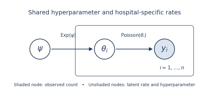
The joint density factors as $p(\psi ){\prod }_{j}p({\theta }_j\mid \psi )p(y_j\mid {\theta }_j)$. In the full conditional distribution of ${\theta }_i$, all factors not involving ${\theta }_i$ cancel. The remaining likelihood function and exponential distribution prior giveIn shape–rate convention this is $\boxed{{\theta }_i\mid \psi ,y\sim \mathrm{Gamma}(y_i+1,1+\psi )}$, a special case of the Gamma–Poisson hierarchical model. It depends only on the node's observed child $y_i$ and parent $\psi$, as required for its Gibbs sampler update.

Integrate the latent variable out to obtain the hospital's marginal likelihood:For $\varphi =(1+\psi {)}^{-1}$ this becomes $\boxed{p(y_i\mid \varphi )=(1-\varphi ){\varphi }^{y_i}}$. It is a geometric distribution on the nonnegative integers, with success probability $1-\varphi$. The transformation concerns the likelihood, so no Jacobian is inserted here.

Put $s={\sum }_i{y}_i$. The independent-count likelihood function is proportional to $(1-\varphi {)}^n{\varphi }^s$. Its conjugate prior is $\boxed{\varphi \sim \mathrm{Beta}(a,b),a,b>0}$, giving the posterior distribution $\mathrm{Beta}(a+s,b+n)$.

A flat density in $\log \psi$ induces $p(\psi )\propto 1/\psi$. Since $\psi =(1-\varphi )/\varphi$, the absolute Jacobian determinant is $|d\psi /d\varphi |={\varphi }^{-2}$. ThereforeThis is the Haldane prior, an improper prior with formal beta parameters $(0,0)$.

Multiplying the likelihood in part (d) by the Haldane prior gives $p(\varphi \mid y)\propto {\varphi }^{s-1}(1-\varphi {)}^{n-1}$. ConsequentlyFor at least one hospital, $n>0$, this posterior is proper exactly when $s>0$. If every count is zero, the kernel diverges at $\varphi =0$ and does not define a posterior distribution; the improper prior cannot then be used for the subsequent expectation.

The gamma full conditional distribution has mean $(y_i+1)/(1+\psi )=(y_i+1)\varphi$. The tower property and the beta distribution mean giveWriting $\overline{y}=s/n$ and $w=s/(s+n)=\overline{y}/(1+\overline{y})$ yieldsThus partial pooling pulls every local mean toward the overall sample mean. The common weight arises from the fixed shape-one mixing distribution; it is the Poisson–exponential posterior shrinkage formula.

The model treats hospitals as exchangeable and assumes the same exponential mixing law for their total expected annual counts. Its shape is fixed: the prior standard deviation equals its mean. Real hospitals differ in size, patient mix, ascertainment and observation effort, so expected counts should not generally share one distribution without accounting for these predictors. Common regional conditions can also invalidate their assumed conditional independence. The resulting geometric distribution for observed counts is a restrictive distributional prediction that can be checked.

Model the count relative to exposure, for exampleHere $E_i$ is a measured exposure such as patient-days, $x_i$ contains hospital predictors, and $b_i$ is a random effect. This Poisson regression separates hospital size from rate variation and supplies partial pooling. Use proper, scale-appropriate priors on coefficients and variation; add regional or temporal effects if the data demand them. A gamma mixing law with an estimated shape is another way to allow more flexible overdispersion. Compare the fitted model's counts and dispersion through posterior predictive checks.