Past exam of the mathematics course of the University of Cambridge / 2009 / iii / Paper 102 (Applied Statistics)

The examination used separately emailed files. For this question a public Guerry data archive and its CSV mirror permit a documented reconstruction: retain the 85 records with a recorded region and select the specified columns. All six printed records match exactly, and each of the five regions has 17 departments. The numerical results below refer to that reconstruction; the remaining rows cannot be checked against the unavailable emailed file.

Treat department identifiers as labels and region as a categorical variable. The following summaries show the scale and spread of the quantitative variables:

A larger population-per-crime value means a lower crime rate, and a smaller wealth rank means greater recorded wealth. Donations are markedly right-skewed, as the large gap between mean and median and the upper tail indicate; rank is an ordinal measure rather than a monetary difference. For the ratio analysed next, the median is $2.683$, the interquartile interval is $[1.829,3.515]$, and the range is $[0.643,10.194]$.

Regional median ratios are $2.763$ in C, $2.502$ in E, $3.979$ in N, $1.373$ in S, and $2.937$ in W. The regional box plots and wealth-versus-log-ratio scatter plot in the figure expose this geographical contrast and an inverse association with wealth rank. North has the highest typical property-to-person crime ratio and South the lowest in the reconstructed data. These summaries are descriptive departmental comparisons, not causal or individual-level conclusions.

If a department has population $P$, $C_{mpers}$ crimes against persons and $C_{mprop}$ crimes against property, cancellation of the common numerator givesThus $y$ is a property-to-person crime count ratio, not its reciprocal. Both counts must be positive for the printed ratio to be defined.

For the reconstructed 85-row data, fit a normal linear model for the Box–Cox transformation $T_{\lambda }(y)$, including four region contrasts plus Literacy, Donations and Wealth. With $z_i(\lambda )=(y_i^{\lambda }-1)/\lambda$ and $z_i(0)=\ln y_i$, the profile likelihood, up to constants, isThe second term is the transformation's Jacobian determinant; omitting it would incorrectly compare different response scales. Maximization gives $\hat{\lambda }=0.143$, with approximate 95% likelihood-ratio confidence interval $[-0.120,0.406]$. The logarithmic transformation is inside this interval, whereas the raw-scale choice $\lambda =1$ is far outside: the twice-log-likelihood drops at zero and one are $1.14$ and $39.54$, respectively. A log-response model is therefore a simple supported choice.

In the full log model, partial F-tests give $F_{4,77}=13.15$ for Region ($p=3.3\times 10^{-8}$), $F_{1,77}=27.99$ for Wealth ($p=1.1\times 10^{-6}$), and $p=0.786,0.682$ for Literacy and Donations. Dropping Literacy and Donations together gives $F_{2,77}=0.109$ and $p=0.897$. A parsimonious final normal linear model, with C as reference and $W=\mathrm{Wealth}/10$, isThe standard errors in that order are $0.1056,0.1105,0.1158,0.1102,0.1104,0.01539$; residual standard deviation is $0.3212$ on 79 degrees of freedom and $R^2=0.626$. Use residual-versus-fitted and quantile-quantile plots, influence diagnostics and checks for remaining curvature to assess the working Gaussian model; the small p-values alone do not validate its assumptions.

Holding Region fixed, worsening wealth rank by ten positions multiplies the fitted conditional median ratio by $e^{-0.08539}=0.918$. Relative to C at the same wealth rank, the fitted median multipliers are $1.081$ for E, $1.375$ for N, $0.563$ for S and $1.212$ for W. Region and wealth rank explain much of the variation; Literacy and Donations add little once those terms are included. These are associations in the reconstructed dataset. Back-transforming the fitted log mean gives a conditional median under lognormal errors; estimating an original-scale mean requires bias correction after an inverse transformation. Also, the public archive's metadata describe some historical measures differently from the exam wording, so the fitted Donations effect is interpreted only on its recorded scale.

Let $S_i$ be singleton deliveries among $C_i$ treatment cycles. Under a common-probability binomial distribution model, $S_i\sim \mathrm{Bin}(C_i,p)$ independently across years. The pooled maximum-likelihood estimator isThe Pearson chi-squared test of homogeneity compares singleton and non-singleton counts across all fourteen years, usingAll expected cells are large. One probability has been estimated, so the reference chi-squared distribution has 13 degrees of freedom. Numerically,The constant singleton-per-cycle probability is decisively rejected under the independent-binomial model. The observed proportion rises from $1712/18201=0.0941$ to $3626/23794=0.1524$. Dependence between repeated treatments or patient heterogeneity can invalidate literal binomial precision, but they should be addressed by an explicit variance model rather than ignored.

Use grouped-binomial logistic regression, $S_i\sim \mathrm{Bin}(C_i,p_i)$ and $\mathrm{logit}(p_i)={\eta }_i$. Center the year as $u_i=i-7.5$. Maximizing $\ell ={\sum }_i[S_i{\eta }_i-C_i\ln (1+e^{{\eta }_i})]$ gives score $X^T(S-Cp)=0$ and information $X^T\mathrm{diag}\{C_i{p}_i(1-p_i)\}X$; these determine the estimates and working covariance matrix.

A straight-line logit fit is $\hat{\eta }=-1.95965+0.045384u$, with naive binomial standard errors $0.005382$ and $0.001352$. Its yearly odds multiplier is $e^{0.045384}=1.04643$, with naive 95% Wald confidence interval $[1.04366,1.04921]$. However, its residual deviance is $58.20$ on 12 degrees of freedom ($p=4.8\times 10^{-8}$), so those small standard errors do not describe an adequate independent-binomial fit.

Comparing polynomial mean structures gives residual deviances $1191.73,58.20,55.70,27.08$ for degrees zero through three, with respective residual degrees of freedom $13,12,11,10$. A quadratic term alone adds little; the cubic structure captures the middle-period acceleration and later leveling. Even the cubic independent-binomial fit has $p=0.00253$ for its residual deviance goodness-of-fit test. A useful working model is therefore cubic quasibinomial regression, retaining the logistic mean and estimating overdispersion rather than claiming an exact binomial law:The Pearson estimate is $\hat{\varphi }=27.182/10=2.718$. Using standard errors multiplied by $\sqrt{\hat{\varphi }}$ and a $t_{10}$ reference, the approximate 95% coefficient intervals are $[-1.98294,-1.92429]$, $[0.04982,0.07445]$, $[-0.001697,0.001131]$, and $[-0.000980,-0.000182]$. An approximate quasi-deviance comparison of cubic against linear gives $F_{2,10}=5.72$ and $p=0.022$, supporting the added shape while acknowledging that only fourteen annual groups inform dispersion.

In this preferred mean model the odds change is not constant:The fitted annual change is larger around the middle than at the ends; the straight-line 4.6% increase is a useful overall summary, not an exact yearly effect in the cubic model. The fitted curve, uncertainty band and residual plot appear in the figure. Singleton success increased overall, but a constant log-odds trend with unit binomial dispersion fits poorly. Quasibinomial intervals remain working-model intervals: serial dependence, changing patient mix and treatment practices cannot be separated from annual aggregates alone.

The correct denominator is the number of live deliveries $B_i=S_i+T_i+H_i$, not treatment cycles and not babies. Define $M_i=T_i+H_i$ and use $M_i\mid B_i\sim \mathrm{Bin}(B_i,q_i)$; this is the distinction in denominators in grouped birth-outcome models. The observed conditional multiple-delivery proportion is $661/2373=0.2786$ initially and $1147/4773=0.2403$ finally.

A constant logit has residual deviance $87.48$ on 13 degrees of freedom. A linear-year fit gives $\hat{\eta }=-1.02533-0.020879u$, deviance $16.46$ on 12 degrees of freedom ($p=0.171$), and annual odds ratio $0.97934$. A quadratic term improves the deviance by $5.814$ on one degree of freedom ($p=0.0159$), whereas a further cubic improvement is only $1.390$ ($p=0.238$). A supported parsimonious binomial model isIts residual deviance is $10.651$ on 11 degrees of freedom ($p=0.473$), and Pearson statistic is $10.647$, with no detected excess dispersion. The binomial standard errors are $0.014445,0.002515,0.000699$; approximate 95% Wald confidence intervals are $[-1.02792,-0.97129]$, $[-0.02496,-0.01510]$, and $[-0.003052,-0.000313]$. The annual odds multiplier is $\exp \{{\beta }_1+{\beta }_2(2u+1)\}$, describing near-flat early behaviour and a stronger later reduction, rather than a uniform annual decrease.

As a secondary check, modelling the triplet-or-higher share alone among deliveries needs curvature: its quadratic logit has residual deviance $12.905$ on 11 degrees of freedom, compared with $92.834$ for a straight line. Multiple delivery became less likely conditional on a live delivery, especially later in the series; higher-order multiples declined particularly strongly. This conditional probability is separate from the probability of any successful live delivery per cycle.

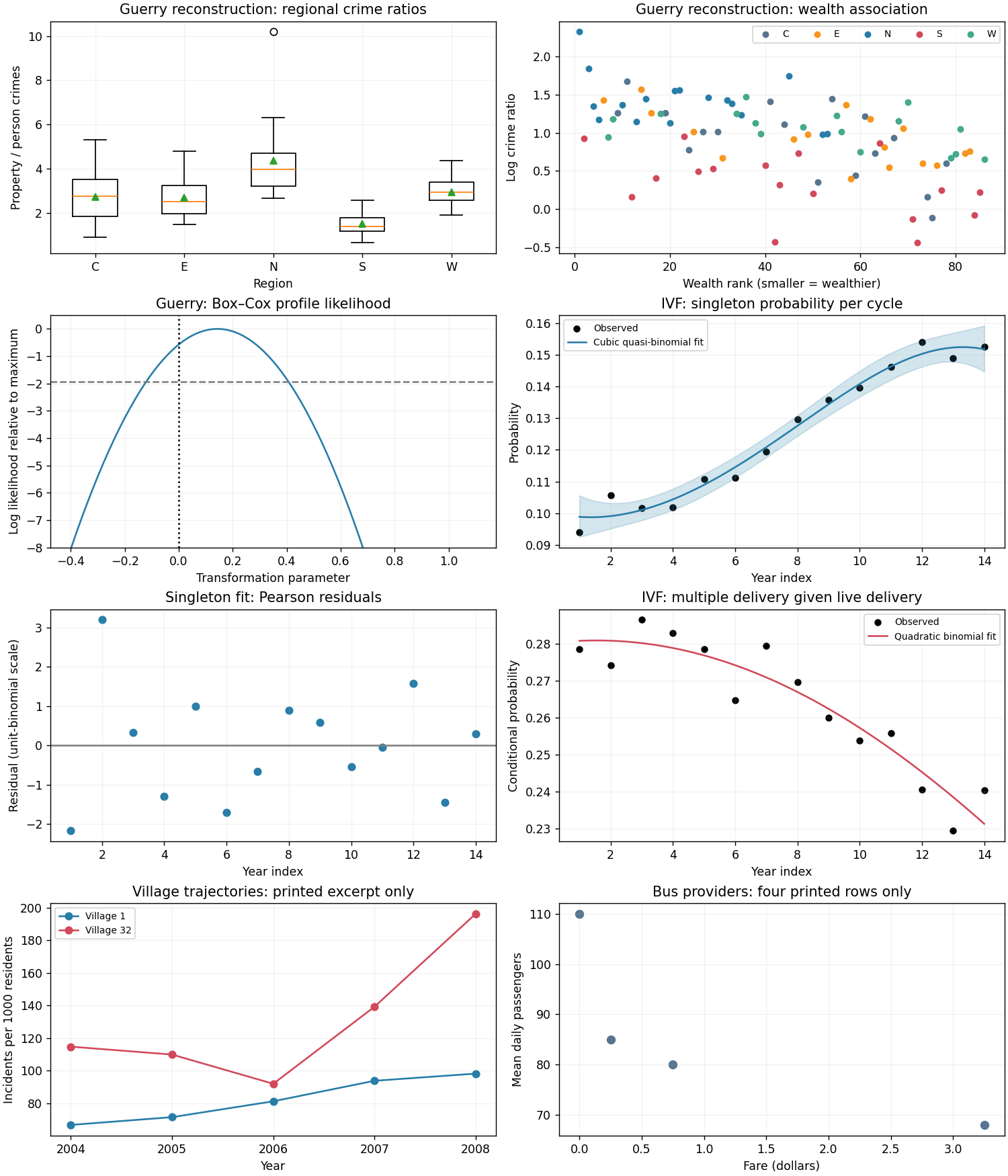
Only four of the twenty provider records are printed, and the full emailed file has not been recovered. The four observed passenger averages have mean $85.75$, median $82.5$, sample standard deviation $17.67$ and range $68$--$110$. Their bus-mile mean is $112.25$, with range $22$--$160$; the highest passenger average belongs to the provider with the lowest bus miles and zero fare. That is a useful diagnostic of differing service patterns, not evidence of a population-wide negative mileage effect.

For the complete dataset, use scatter plots of passenger average against bus miles, fare and population, and inspect population-scaled demographic counts as well as their raw counts. Compare marginal distributions and the sample correlation matrix, especially among population, older residents, low-income households and poverty households: these measure overlapping aspects of area size and composition and can create multicollinearity. Inspect the zero fare directly; a logarithm of fare is undefined there, so do not silently drop it. All four displayed rows belong to the fixed-route group, so they cannot support a between-service comparison.

The figure labels its bus panel as a four-row excerpt. Twenty-provider summaries and exploratory conclusions cannot be determined from these four rows. In particular a full eight-parameter regression has more parameters than observed rows; reporting a fitted full-data model from this excerpt would be unjustified.

Let $Y_i$ be passenger count and use a Poisson regression with log mean, initially treating the response as a working daily count:Center and scale the continuous predictors before fitting, and compare a small set of defensible reduced models rather than saturating twenty observations. Household counts should not be called household proportions without a household denominator; population-scaled counts are alternative intensity covariates. Bus miles can be an estimated elasticity term rather than an offset, since proportionality of passenger numbers to bus miles has not been established.

For actual counts, the log-likelihood score is $X^T(Y-\mu )=0$, with ${\mu }_i=e^{x_i^T\beta }$. Fitting by iteratively reweighted least squares uses weights ${\mu }_i$ and working response ${\eta }_i+(Y_i-{\mu }_i)/{\mu }_i$. Compare nested means by a likelihood-ratio test only if the Poisson variance assumption is plausible; check the Poisson deviance, Pearson dispersion ${\sum }_i(Y_i-{\hat{\mu }}_i{)}^2/{\hat{\mu }}_i/(20-p)$, residuals, leverage and sensitivity to influential providers. Consider Quasi-Poisson regression or negative binomial regression if variance exceeds the mean.

The recorded response is actually a daily average, so Poisson working models for averaged counts need special care. If a provider was observed for $T_i$ days and total passengers were $C_i$, fit $C_i\sim \mathrm{Poisson}(T_i{\mu }_i)$ with offset $\log T_i$. If only the average and no observation duration are available, a Poisson mean model can still be explored, but its likelihood and standard errors are not automatically justified by integer-looking averages.

A one-unit increase in an untransformed predictor has fitted multiplicative mean effect $e^{{\beta }_j}$; a bus-mile elasticity ${\beta }_B$ gives a doubling effect $2^{{\beta }_B}$. No numerical coefficient estimates or selected twenty-provider model are identifiable from the printed excerpt. The full provider file and, ideally, the averaging periods are needed to execute these model comparisons.

Preserve the original row order and set $G_i=0$ for the first eight fixed-route providers and $G_i=1$ for the twelve on-demand providers. A suitable group comparison builds on a selected small predictor set $z_i$:The model with $\gamma =0,\delta =0$ pools service types; adding $\gamma$ changes the baseline; adding selected components of $\delta$ allows different predictor dependence. Center $z$ at meaningful values so that $e^{\gamma }$ compares groups at those values. The predictor-specific rate ratio is $e^{{\beta }_j}$ in the fixed-route group and $e^{{\beta }_j+{\delta }_j}$ in the on-demand group; the group ratio at predictor value $z$ is $e^{\gamma +z^T\delta }$.

Fit common-slope and selected-interaction models, respecting model hierarchy by retaining corresponding main effects. Test the added interaction block jointly with a likelihood-ratio test, or an appropriate quasi-likelihood comparison under estimated dispersion, and check group-specific residual patterns and leave-one-provider sensitivity. Seven interactions plus all main effects would use 16 parameters for just twenty providers and leave only four residual degrees of freedom; an indiscriminate full interaction model is consequently a poor basis for stable inference.

The excerpt contains only $G=0$, so neither the service-type effect nor any interaction is estimable from it. Full-data estimates could distinguish a baseline difference from genuinely different slopes, but the printed records cannot establish either conclusion.

Use incident counts $Y_{it}$ divided by that village-year's population exposure $P_{it}$, and graph $r_{it}=1000Y_{it}/P_{it}$ against calendar year. Show separate small panels or labelled lines for all villages; a population-weighted overall line answers a different question from an equally weighted average village rate. A plot of counts alone can mistake population change for a rate change.

For the two printed villages, the observed rates per thousand residents are approximatelyThe first trajectory increases throughout; the second falls initially and then rises sharply. The last-to-first rate ratios are $1.472$ and $1.711$, respectively. The figure displays these two observed trajectories only. The other thirty village trajectories cannot be drawn from the PDF, because their observations were supplied in the separate emailed dataset.

For a population-averaged rate trend, use the marginal incidence trend with clustered observations modelFit a generalized estimating equation with village as cluster, a log link and an appropriate working correlation; estimate uncertainty with a village-level sandwich covariance matrix. Then $e^{\beta }$ is the fitted annual marginal rate ratio, $100(e^{\beta }-1)$ is the annual percentage rate change, and $e^{4\beta }$ is the four-year endpoint ratio. Test $\beta =0$ using cluster-robust uncertainty, with a small-sample correction or village-resampling bootstrap given only 32 independent clusters. Also compare year as a factor with a linear trend, since a single slope can conceal nonlinear behaviour.

Report which population is averaged over. The directly pooled rate ${\sum }_i{Y}_{it}/{\sum }_i{P}_{it}$ is exposure weighted; a mean of village rates gives each village equal weight. For standardized comparisons one can use the same village weights at every year, preventing changing population composition from masquerading as a rate trend.

A conditional random-slope coefficient cannot simply be substituted for the marginal slope: the marginal mean of a Poisson random-slope model contains time-dependent variance terms. A direction, magnitude and confidence interval for the trend across all villages require the missing full dataset. The increase in the two displayed villages does not determine the trend in the other thirty.

Center time at 2008 by setting $s=t-4$, and initially ignore the explanatory covariates. A Poisson generalized linear mixed model addressing both heterogeneity questions isHere ${\tau }_0$ describes between-village variation of log rates in 2008, while ${\tau }_1$ describes heterogeneity of annual log-rate changes. The latent 2008 rate has median $e^{{\beta }_0}$, mean $e^{{\beta }_0+{\tau }_0^2/2}$ and coefficient of variation $\sqrt{e^{{\tau }_0^2}-1}$. A central 95% interval for latent village rates is $e^{{\beta }_0\pm 1.96{\tau }_0}$; the corresponding interval for village-specific annual rate ratios is $e^{{\beta }_1\pm 1.96{\tau }_1}$. These describe heterogeneity, not confidence intervals for estimated fixed effects.

Fit an intercept-only random-effects model and then add a correlated random slope. Compare them with a parametric bootstrap of the likelihood improvement: the null slope variance is on the boundary, so an ordinary fixed-effect chi-squared reference is not automatically valid. Inspect uncertainty in both variance components, shrinkage of village-specific estimates, residual overdispersion and remaining serial correlation. A negative-binomial conditional model can distinguish additional within-village count variation from persistent village differences when the data support it.

By the marginal mean of a Poisson random-slope model, the marginal log rate is ${\beta }_0+{\beta }_{1}s+({\tau }_0^2+2s{\tau }_{01}+s^2{\tau }_1^2)/2$, so marginal curvature can arise even when each village has a straight conditional log trend. Numerical variance estimates and evidence of heterogeneous slopes cannot be obtained for 32 villages from two displayed trajectories.

Use the population as exposure regardless of whether a population-size category is also a covariate. Define a demographic factor with levels $\mathrm{Low}$ for at most 20%, $\mathrm{Medium}$ for $(20,30]$%, and $\mathrm{High}$ above 30%; define $H_{it}=1_{\{P_{it}>250\}}$ if following the suggested population dichotomy. Treat village-size codes as a categorical variable, not equally spaced areas.

A candidate multivariate Poisson generalized linear mixed model retains the random intercept and slope from part (c) and usesThis specifies the suggested village-size-by-population interaction while keeping its main effects. One may add selected time-by-covariate interactions to explain slope heterogeneity, provided information from 32 clusters supports them. Compare continuous demographic and population formulations as a sensitivity analysis: categorization loses information, and the coefficient of a size category measures association beyond the already included exposure effect.

Fit models with the same likelihood convention and conditional distribution when comparing Akaike information criteria; use joint fixed-effect likelihood-ratio tests, boundary-aware parametric bootstrap tests for random effects, residual diagnostics and village-level cross-validation to justify a parsimonious final model. Preserve interactions' main effects and report interval estimates from the final multivariate model, rather than interpreting separate univariate fits. For example, the adjusted inland-versus-coastal rate ratio is $e^{{\theta }_I}$, while a medium-versus-small village ratio is $e^{{\gamma }_2+{\kappa }_{2}H}$; a Wald interval for that contrast uses the full coefficient covariance matrix. Conditional time effects and standardized marginal predictions should be distinguished.

The displayed rows cannot identify this final model: population exceeds 250 in every displayed village-year, no large village is shown, and inland status is confounded with the identity of the two displayed villages. The complete 160-row file is needed for fitted effects, model selection, all-village plots and uncertainty. No numerical best model or evidence of the specified covariate associations can honestly be reported from this excerpt.

Finally, even a significant adjusted association with young-male percentage would not show that young males were involved in most incidents. This is the ecological fallacy, specifically that aggregate composition does not identify offender composition: the same village counts can be assigned to different individual age and sex groups without changing any observed aggregate predictor. Individual incident-level age, sex and involvement records are required to answer that last question. The aggregate dataset cannot establish the claimed majority involvement.