Let be the flight distance in millimetres for paper level , launch-angle level , design level and replicate , where and . The full factorial design is fitted by the normal linear modelThe assumptions are independent errors with a common variance and normal distribution, and the displayed factor-combination mean structure. The corner-point constraints areand whenever at least one index equals . Thus the eight free mean coefficients are . These treatment coding coefficients are comparisons at the other factors' reference levels, rather than necessarily averaged main effects.
To test the three-factor interaction term, compare the full model with the model retaining all main effects and all two-factor interactions. The null hypothesis is , against a nonzero value. Removing it increases the residual sum of squares by and removes one parameter. With eight residual degrees of freedom, the nested-model F-test givesThere is no evidence that this three-factor interaction is needed. This does not establish that all two-factor interactions vanish: the paper-design interaction is substantial.
The
stepAIC command performs stepwise selection by the Akaike information criterion. Its upper scope is the full factorial model and its lower scope is the intercept-only model. Starting from the full model, it compares admissible additions and deletions, preserving the hierarchy of interaction terms, and chooses changes that reduce the Akaike information criterion. With the supplied scope its default search permits both directions. For these Gaussian fits the displayed criterion, up to constants common to all models, is , where counts mean coefficients. The first deletion changes it from to : the small increase in residual sum of squares is outweighed by removing a parameter. This is a greedy model selection procedure, not an exhaustive search or a sequence of fixed-level hypothesis tests. The command's arguments are described in the MASS documentation.For the selected model, let and . Thenindependently between flights. It has no angle term. The maximum-likelihood estimates of its mean coefficients are also obtained by ordinary least squares:For example, the four fitted means are just the four paper-design cell means, each averaging four flights over the angle levels. With , the variance-covariance matrix of the coefficient estimates is . Its diagonal gives the displayed standard errors; their ratios are , with mm.
The final line of
summary(model2.lm) is the joint nested-model F-test of , comparing this four-parameter model with a common mean. Its statistic iswith F-distribution under the fixed-model null and P-value . Thus the selected paper-design terms jointly improve the fit substantially. The coefficient of determination means they account for about of the observed centred variation. These nominal inferential summaries do not adjust for the preceding model selection on the same data.Using the unrounded fitted means givesin millimetres. Hence choose the high-performance design with the lighter paper; the fitted model leaves both launch angles tied, with expected distance about mm. A preference for one angle is not supported by this selected model. The strong paper-design interaction reverses the design comparison: the simple design is better on heavy paper, whereas the high-performance design is better on light paper. Consequently a single design effect averaged over paper types would conceal the main result. There is little evidence here for an angle effect, and considerable flight-to-flight variability remains.
Before fitting, inspect raw-distance dot plots for all eight factor combinations, and interaction plots of cell means against design, with separate lines for paper and panels for angle. With only two replicates per cell, showing individual observations is more informative than elaborate box plots. These reveal reversals, spread and possible unusual flights. Afterwards inspect a residual-versus-fitted plot, a Q-Q plot of residuals, a scale-location plot, residuals against each factor and, if recorded, flight order, and Cook's distance for influential observations. Residual patterns by angle would question its deletion, while unequal spread or departures from the normal distribution would question the error assumptions rather than merely demand another mean term.
Work at a regular admissible parameter value with , so the score identities in the question apply. For one observation from the exponential dispersion family, the score function and second derivative areThe zero expected score immediately gives . The equality between expected negative curvature and score variance then givesThusThe admissible density parameters necessarily make this variance nonnegative; the algebra does not require an unstated sign assumption beyond the regular family and .
With independent observations and canonical parameters , the chain rule gives the vector score functionA finite interior maximum-likelihood estimator satisfies its score equation, provingDifferentiating again, using , givesThis Hessian is independent of the observations, so taking expectation gives exactly the requested Fisher information matrix. In particular, is not the inverse observation-variance matrix: the linear predictor here is the canonical parameter, not the mean.
For the two-group Poisson regression, , , and . Put , , using here for the second group's mean. There are observations, andHence the total Fisher information matrix and its inverse areThe theorem on asymptotic normality of a maximum likelihood estimator says that in a regular identifiable model with nonsingular information the estimator is approximately multivariate normal, centred at the true parameter and with covariance equal to the inverse total information. Here one can regard one observation from each group as an independent pair and apply its usual iid version to such pairs. ThereforeFor a direct check, the second score equation gives the fitted second-group mean , and the first then gives the fitted first-group mean . Thus the Poisson log-rate ratio estimate is . The delta method, using independent sample-mean variances and , gives the same variance . If a group total is zero, its finite log-mean estimator fails to exist; with fixed positive true means this event has probability tending to zero exponentially as grows.
Let be the disease count among miners in exposure group , with representative exposure , for . The grouped-binomial logistic regression isThe model assumes independent miners, a common disease probability within each group at its representative exposure, and binomial variation without an extra dispersion parameter. The use of average exposure is a grouping approximation, not a claim that every miner in a group has identical exposure. The input response is and
weights=miners supplies the binomial denominators , not inverse variances; together they yield this count likelihood function. The default binomial link is the logit link.For , the likelihood-ratio test compares the intercept-only model with the linear-exposure model. The reduction in binomial deviance isUnder the usual regular large-sample approximation it has a chi-squared distribution with one degree of freedom. There is very strong evidence of exposure dependence, with a positive estimated coefficient .
For goodness of fit against separate probabilities in all eight groups, the residual binomial deviance has approximately degrees of freedom. Its upper-tail probability is about , giving no evidence of lack of fit. This is an approximate check, particularly because the earliest exposure groups have small expected disease counts. It supports adequacy of this mean structure, not proof that all its assumptions or possible confounding variables have been addressed.
The
predict call asks for a prediction at exposure , sets type="response" to return the fitted probability rather than its log odds, and requests the standard error of that fitted probability. It givesFor , the linear predictor is , and the delta method givesThe intercept-slope covariance is included in this expression. This measures uncertainty in the fitted mean probability; it is not the standard deviation of a new individual's binary disease outcome or of an unspecified new sample proportion.The model's odds at exposure are . Hence , independently of . By invariance of maximum likelihood estimation, estimate this odds ratio by . A Wald confidence interval for is ; exponentiating its endpoints after multiplication by gives the interval for the multiplier. Using the printed coefficient and standard error yieldsThus the estimated odds rise by about per year, or by a factor about per decade. These are changes in odds, not fixed multiplicative changes in probabilities.
The second fit keeps the same independent binomial distributions but permits a quadratic linear predictor,In the sequential analysis, each exposure term adds one coefficient. With the first model's deviances, all nine missing entries are recovered in this completed table:The final reduction is , with rounding to the precision of the printed output. Testing therefore gives on one degree of freedom. At the significance level I would retain the simpler linear-exposure model: it already fits adequately and the extra curvature is not clearly established. The quadratic fit does improve the likelihood somewhat; its Akaike information criterion is about smaller, since . Thus different reasonable selection criteria may weakly prefer different models, but these data do not give strong evidence that the additional term is necessary.
For the one-sided Wilcoxon rank sum test, suppose and are independent samples, iid within each sample, with continuous distributions. The null hypothesis is a common distribution. For a lower-tail alternative, the distribution is stochastically smaller. In the common-shape location model , this is against ; in that model it also compares medians. Without a location-family assumption, equality or inequality of medians alone is not the defining rank-sum hypothesis.
Rank all observations from smallest to largest and form . Reject for small . Under , the labels are exchangeable, so every subset of of the ranks is equally probable. The exact null distribution of a rank sum is thereforeEnumerate these subsets, or use the coefficient of in . An efficient recursion adds rank either to the selected sample or not: , starting with . The lower-tail P-value is . A nonrandomized level- test chooses a lower-tail rejection region whose null probability is at most .
The shifted Mann–Whitney U test statistic is . It counts pairs with , so the same lower-tail test uses small . The distinction is important for these S-Plus outputs: the printed values are raw rank sums, not the shifted statistic used by some other software.
For the one-sided Wilcoxon signed-rank test, the pairs are independent between individuals but their two measurements may be dependent. Let , and assume the differences are iid, continuous and symmetric about a common location . Test against . Rank the absolute differences and useUnder the null, conditional on their absolute values, the signs are independent fair signs. Every subset of ranks therefore has probability of being the positive-sign subset, giving the exact null distribution of . Reject for small and calculate the lower-tail probability. Its null mean and variance are and . The symmetry assumption is essential: zero median by itself does not give this law. With zeros or ties, omit zero differences in the usual signed-rank version and use average ranks for ties, adjusting the distribution accordingly. The paired test is not appropriate for the independent RHR samples here.
For the experienced participants, let denote RHR1 running time and denote RHR2 running time. The null hypothesis is identical running-time distributions; under the location interpretation it is zero RHR1-minus-RHR2 shift. The one-sided alternative is a negative shift, so RHR1 participants tend to run faster. With , the printed statistic isAt , reject the null in favour of faster RHR1 running times. The sample medians and minutes agree with that direction; their difference is descriptive, not the rank-sum test statistic.
For the new participants the same independent-sample Wilcoxon rank sum test compares eight RHR1 times against nine RHR2 times, again with a lower-tail alternative. HereThe exact null distribution of a rank sum gives this probability. It does not reject at , although it is just below . The data suggest the same direction but are less decisive; this is not evidence that the two new-participant distributions are equal.
The final command pools the experienced and new RHR1 samples into observations, and the corresponding RHR2 samples into . It repeats the lower-tail rank-sum comparison on these two pooled groups.
exact=F requests a normal approximation for a rank sum with a continuity correction. Without ties,The lower-tail statistic is , with the usual tie-adjusted variance if ties occur. The supplied output iswhere is the standard normal distribution function. Thus the pooled test rejects at . The unreported pooled ranks must be formed afresh: the within-cohort raw rank sums cannot simply be added because pooling introduces cross-cohort comparisons.Taken together, there is evidence that participants classified as RHR1 have shorter running times among the experienced men and in the pooled sample. The smaller new-participant samples give weaker evidence in the same direction. A significant result in one cohort and a nonsignificant result in another does not itself prove that their RHR effects differ. Pooling also assumes a meaningful pooled comparison; if programme duration changes the distributions, a cohort-adjusted analysis would be more informative. These observational comparisons do not establish that the fitness programme caused the differences, and none of the three tests directly compares experienced participants with new participants.
The fitted continuous-time multi-state model allows only adjacent fatigue-state jumps. Its four transition intensities, in reciprocal years, are shown here:
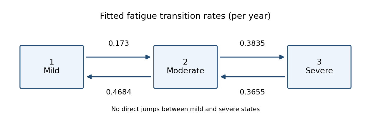
Estimated fatigue transition intensities: mild to moderate 0.173, moderate to mild 0.4684, moderate to severe 0.3835, and severe to moderate 0.3655 per year
. Details. 
In state , the total exit intensity is . By the holding time law for a continuous-time Markov chain, the time until the next jump has an exponential distribution with this rate. ThereforeThe printed interval for gives the interval for . Taking reciprocals reverses the endpoints, so the transformed confidence interval for the mean holding time isFor the next jump's destination, competing outgoing intensities giveIndeed the density of a first jump to at time is ; integrating gives the ratio above. This is a conditional next-jump probability, not a transition probability of being mild at a fixed later visit.
The command uses the model without covariates, starts in mild fatigue at time zero, and calculates expected accumulated years in each state between times and . Let be the fatigue state and its fitted generator matrix. For the occupation time of a continuous-time Markov chain,the expected finite-horizon occupation time isThe first equality follows by interchanging a bounded time integral and expected value, and the second uses the homogeneous continuous-time Markov chain transition matrix. The reported expectations are 7.014800 years mild, 1.724686 years moderate, and 1.260514 years severe. They sum to ten because the person occupies exactly one state at every time. All repeated entries are counted: these are not the lengths of single holding times, the durations until first reaching each state, or the probabilities of occupying the states at year ten. The interpretation of the time limits is also given in the package documentation.
For patient , let be the fatigue state at time years since study entry. Let the covariate vector be , representing the sex indicator, arthritis duration in years, HAQ disability score and haemoglobin measurement. Conditional on these covariates, the continuous-time multi-state model has the Markov property and generator matrixEach allowed transition intensity has its own log-linear transition intensity model, . The zero entries exclude direct instantaneous jumps between mild and severe states, and the diagonals enforce zero row sums.
To express the estimates correctly, the printed intensities are evaluated at the sample covariate means , not at . Order the allowed transitions as . Their estimates arewith rows indexed by that transition order and columns by inEquivalently, the uncentred intercept is . The means are not printed, so the displayed rates cannot be treated as numerical zero-covariate intercepts.
The assumptions are independent patients conditional on their covariates; correctly observed fatigue states; no unmodelled history dependence once current state and covariates are known; positive adjacent-state intensities with the specified exponential covariate dependence and no interaction terms; and a noninformative observation and censoring mechanism for the conditional state-process likelihood. With fixed covariates the rates are homogeneous in time and holding times are exponential. Covariates updated at visits are treated as piecewise constant between observations, so each such interval has a constant generator, a piecewise-constant covariate approximation. In particular this is an approximation if a quantity such as duration changes continuously between visits.
For observations , conditioning on the initial observed state, the panel-observed multi-state likelihood is a product over patients and intervals ofwhere is the covariate value held over that interval. Multiple unobserved jumps within an interval are integrated out by this transition matrix. For example, a mild state followed by a severe state can have positive likelihood despite , because an unobserved moderate state can intervene. The panel observations within a patient are not independent; it is the Markov property that justifies multiplying conditional transition probabilities. The piecewise-constant handling of changing covariates is specified in the msm model documentation.
For the mild-to-moderate transition intensity, an increment in a single covariate, with the others held fixed, gives the multiplicative ratio . Of the four printed effects on this transition, sex and HAQ have confidence intervals excluding zero on the log-intensity scale.
With male coded and female coded , the estimated hazard ratio for males relative to females isThus, conditional on currently being mildly fatigued and on the other covariates, males have an estimated mild-to-moderate transition intensity about lower than females. The conclusion concerns this particular instantaneous transition, rather than a general reduction in fatigue probability.
For a one-point increase in HAQ, indicating greater physical disability, the estimated intensity multiplier isGreater disability is therefore associated with a substantially faster mild-to-moderate transition, after adjustment for sex, arthritis duration and haemoglobin. Both conclusions use the specified log-linear transition intensity model and the nominal individual intervals. Arthritis duration and haemoglobin have intervals including zero for this transition, so their effects here are not statistically significant at ; this says neither that their effects are zero nor that they are insignificant for all other transitions.
Articles by others on the same topic
There are currently no matching articles.