Past exam of the mathematics course of the University of Cambridge / 2012 / iii / Paper 37 / 5

Right censoring occurs when a subject's exact failure time $T$ is unobserved but it is known that $T>C$, where $C$ is the censoring time. The observed pair is $U=\min (T,C)$ and $\Delta =1_{\{T\le C\}}$. For example, a living participant at study closure contributes a survival lower bound rather than a recorded death at closure. Right censoring differs from simply omitting the subject: time spent in the risk set remains informative.

A standard sufficient non-informative censoring assumption is independent censoring: $T$ and $C$ are independent, or conditionally independent given the covariates used in the analysis. Their distributions need not be equal, have the same shape, or have proportional hazards. In a likelihood analysis the censoring distribution should also carry no information about the survival parameters being estimated, allowing its factor to be omitted. In the more general risk-set formulation, the censoring history must not alter the subsequent failure hazard conditional on the observed history used by the model. Informative censoring can arise if worsening unrecorded health causes withdrawal.

Among subjects alive at any given time and with the same relevant covariates or observed history, those censored at that time have the same subsequent failure distribution as those who remain under observation. Equivalently, the observed risk set represents the failure hazard of comparable subjects still alive, rather than selectively retaining lower- or higher-risk subjects. This is a statement about their future conditional risk, not that the observed failure-time distribution among censored people equals the distribution among people who eventually fail: their different observation patterns make that comparison inappropriate.

Let $f_j=\mathbb{P}(T=t_j)$ and $h_j=\mathbb{P}(T=t_j\mid T>t_{j-1})$. Since $S(t_{j-1})=\mathbb{P}(T>t_{j-1})$, the discrete hazard satisfies $h_j=f_j/S(t_{j-1})$. HenceStarting from $S(0)=1$ and iterating, the survival function isUnder independent censoring, the risk set just before $t_j$ gives the binomial conditional failure likelihood $h_j^{d_j}(1-h_j{)}^{n_j-d_j}$, whose maximizer is ${\hat{h}}_j=d_j/n_j$. This gives the Kaplan–Meier estimatorFailures at exactly $t$ are included because the target is $\mathbb{P}(T>t)$. Censored subjects contribute to earlier risk sets and leave before later ones; they do not create a failure factor. The usual convention includes a subject censored at a tied failure time in the risk set for that failure. Estimation beyond the last observed failure is limited by the available follow-up.

The last lung-cancer failure before five years is at 4.85, where the displayed net survival estimate is 0.392. The other-death net survival estimate remains 0.498 from 4.096 until 5.065. Thus the two supplied curves imply net five-year death estimates of $1-0.392=0.608$ for lung cancer and $1-0.498=0.502$ for other causes. Their sum is 1.110, already showing that they cannot be probabilities of two disjoint actual causes of death.

In competing risks, let ${\lambda }_1(t)$ and ${\lambda }_2(t)$ be the cause-specific hazards while alive, with cumulative hazards ${\Lambda }_k(t)={\int }_0^t{\lambda }_k(u)du$. Treating the other cause as censored estimates the net survival $S_k^{\mathrm{net}}(t)=e^{-{\Lambda }_k(t)}$. The actual probability of death from cause $k$ by time $t$ is the cumulative incidence functionSince $S(u)\le e^{-{\Lambda }_k(u)}$, the net probability $1-S_k^{\mathrm{net}}(t)$ generally overstates the cumulative incidence function: death from the other cause prevents a later death of cause $k$. This discrepancy exists even for independent latent cause-specific failure times. Moreover, Kaplan–Meier estimates are not generally exactly unbiased in finite samples even for their proper target. The plotted complements are not unbiased estimators of $\mathbb{P}(T\le 5,D=k)$, and are not even consistent for that target in general.

For the desired probabilities, use the Aalen–Johansen estimator ${\hat{F}}_k(t)={\sum }_{u\le t}\hat{S}(u-)d_k(u)/n(u)$, with all-cause survival $\hat{S}(u)={\prod }_{v\le u}[1-(d_1(v)+d_2(v))/n(v)]$ and independent study censoring. Removing competing deaths from subsequent risk sets is correct for estimating cause-specific hazards; the error is interpreting the separate net survival complements as cumulative incidence functions. A hypothetical elimination-of-a-cause interpretation of net survival would require additional causal assumptions.

Use the three-state competing risks model shown below. State 0 is alive after surgery, state 1 is dead from lung cancer, and state 2 is dead from other causes. Both death states are absorbing. Study censoring is an observation mechanism, not a biological transition to a fourth state.

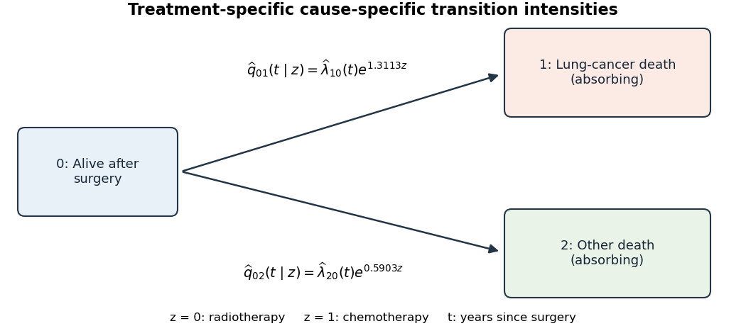
For treatment $z=0$ (radiotherapy) or $z=1$ (chemotherapy), define the transition intensityThe fitted Cox proportional-hazards models areHere ${\hat{\lambda }}_{10}$ and ${\hat{\lambda }}_{20}$ represent the estimated baseline cause-specific hazards for radiotherapy. More formally, the baseline estimates can be expressed as cumulative hazard measures with increments $d_k(t)/{\sum }_{i\in R(t)}{e}^{{\hat{\gamma }}_k{z}_i}$, rather than ordinary smooth functions. All outgoing intensities from states 1 and 2 vanish, and $q_{00}=-(q_{01}+q_{02})$. The treatment hazard ratios are 3.7111 and 1.8045 respectively. This model describes the two observed causes of death, not identifiable latent failure times after death has already occurred.

Among patients still alive at the same time after surgery, chemotherapy has an estimated lung-cancer death rate 3.71 times that of radiotherapy, assuming proportional cause-specific hazards. The estimated 95% confidence interval for this hazard ratio is $(1.583,8.697)$. Thus the fit suggests a higher instantaneous lung-cancer death rate on chemotherapy, with appreciable uncertainty in its size.

The null hypothesis of no treatment effect on that hazard is $H_0:{\gamma }_1=0$ against ${\gamma }_1\ne 0$. Its Wald test uses $Z=1.3113/0.4346\simeq 3.018$, approximately standard normal under the null hypothesis, with two-sided $p=0.00255$. This is evidence against equal lung-cancer death hazards in the fitted model. It is not a statement that five-year lung-cancer death probability is multiplied by 3.71 or that survival duration is divided by 3.71. The cumulative incidence function depends on both cause-specific hazards, and the model needs proportional-hazards and independent observation-censoring assumptions. In a randomised comparison the assigned treatment contrast is protected against baseline confounding, but the instantaneous comparison concerns the groups who have survived to the time in question; it does not identify a treatment effect within a common latent survivor subgroup.