Past exam of the mathematics course of the University of Cambridge / 2012 / iii / Paper 37 (Applied Statistics)

Use the normal linear model $Y=X\beta +\epsilon$, with fixed full-column-rank design matrix $X$, independent errors ${\epsilon }_i\sim N(0,{\sigma }^2)$, and ${\sigma }^2>0$. Its log-likelihood isFor fixed ${\sigma }^2$, differentiating with respect to $\beta$ gives $X^T(Y-X\hat{\beta })=0$. Since $X^{T}X$ is positive-definite, the unique least-squares estimate isLet $\mathrm{RSS}=\Vert Y-X\hat{\beta }{\Vert }^2$. The variance score equation is $-n/(2{\sigma }^2)+\mathrm{RSS}/(2{\sigma }^4)=0$, givingThis is the maximum-likelihood estimator, whereas the residual standard error reported by linear-regression software is $s=\sqrt{\mathrm{RSS}/(n-p)}$. The latter uses the unbiased residual estimate of Gaussian noise variance. These formulas assume $n>p$ and positive RSS; exact interpolation gives a variance-boundary degeneracy rather than an interior maximum.

The regression residual vector is $e=Y-X\hat{\beta }=(I-H)Y$, where $H=X(X^{T}X{)}^{-1}{X}^T$ is the hat matrix. Both $H$ and $I-H$ are symmetric idempotent matrices, and $(I-H)X=0$. Therefore $e=(I-H)\epsilon$ and the linear image of a multivariate normal vector givesThis multivariate normal distribution is singular, with rank $n-p$: fitted-residual orthogonality forces $X^{T}e=0$. Specifically, $\mathrm{Var}(e_i)={\sigma }^2(1-h_{ii})$ and $\mathrm{Cov}(e_i,e_j)=-{\sigma }^2{h}_{ij}$ for distinct observations. Thus regression residuals are generally neither independent nor identically distributed, even though the model errors are. Also $\mathrm{RSS}/{\sigma }^2\sim {\chi }_{n-p}^2$ and is independent of $\hat{\beta }$, which justifies the standard errors and exact Student t-tests below.

In an R formula, I(...) protects ordinary arithmetic from the formula operators: the predictor is the numerical variable $z=x-165$, rather than an instruction to remove a formula term. Predictor centering leaves fitted values and the height slope unchanged but places the intercept at a meaningful height. It often reduces the correlation between intercept and slope estimates.

With $M_i=1_{\{i=2\}}$, treatment contrasts use female as the reference level in a regression factor. The fitted normal linear model isThe estimates and their standard errors areThe intercept estimates female mean weight at height 165. At that same height the male fitted mean is $58.4711+4.3294=62.8005$. Holding height fixed, the fitted male mean exceeds the female mean by 4.3294 weight units. Within either sex, one additional height unit increases fitted mean weight by 0.6211 weight units. If height is in centimetres and weight in kilograms, these interpretations use centimetres and kilograms accordingly. A standard error for the male intercept would require the covariance between ${\hat{\beta }}_0$ and ${\hat{\beta }}_M$, which is not printed.

The prediction equation is $\hat{Y}=58.4711+4.3294M+0.6211(x-165)$. Predictions for individual students also have residual uncertainty, estimated by $s=5.710$, beyond uncertainty in the fitted mean.

The additive model gives useful evidence for both predictors. To test for no adjusted sex effect, use $H_0:{\beta }_M=0$ against $H_1:{\beta }_M\ne 0$. The statistic $T={\hat{\beta }}_M/\mathrm{se}({\hat{\beta }}_M)$ has a Student t-distribution with 97 statistical degrees of freedom under the normal linear model and the null hypothesis. Here $T=3.016$ and $p=0.00327$. Similarly, $H_0:{\beta }_h=0$ against a nonzero common slope gives $T=4.397\sim t_{97}$ under the null hypothesis, with $p=2.81\times 10^{-5}$. Thus, at a fixed height males have a higher fitted mean weight, and within sex greater height is associated with greater weight.

The interaction model adds $\delta M(x-165)$. Its female height slope is $0.6696$ and its male height slope is $0.6696-0.0977=0.5719$. Test $H_0:\delta =0$ against $H_1:\delta \ne 0$ using $T=-0.344\sim t_{96}$ under the null hypothesis, or equivalently $T^2\sim F_{1,96}$. The $p$-value is 0.73139. The additive model is a reasonable parsimonious choice; the data give no evidence for different height slopes between sexes. This does not establish exact equality of population slopes. The additive model also has the higher adjusted coefficient of determination, 0.405 versus 0.3996, and a slightly smaller residual standard error.

Ignoring sex gives a height slope of 0.8769, appreciably above the adjusted slope 0.6211. This is omitted-variable bias in the descriptive regression: a taller group with a larger intercept makes the pooled height association steeper. Algebraically, with $z=x-165$,The printed estimates imply a positive height-sex covariance. Pooled and adjusted slopes therefore describe different comparisons; the difference is not evidence that adding sex changed a physical effect of height. For predictions, retain both sex and height, check regression diagnostics, and assess performance on new students. The residual standard error near 5.7 remains substantial and the coefficient of determination near 0.42 does not promise precise individual prediction.

The largest positive regression residual divided by the residual standard error is about $26.6071/5.942=4.48$, $24.7151/5.710=4.33$, and $24.5908/5.737=4.29$ in the three models. In comparison, the most negative regression residual is only about two residual standard errors below zero. At least one observation is much heavier than its fitted value, even after adjusting for sex and height.

A standardized regression residual is $e_i/[s\sqrt{1-h_{ii}}]$, so the regression leverage adjustment can make these ratios larger. The maximum is selected among 100 correlated regression residuals, however; it is not a prespecified single standard-normal observation. These summaries do not give a formal regression outlier test or identify which student is extreme. Ask to check the measurement and data entry, examine residual plots and a normal quantile-quantile plot, and inspect regression leverage and influential observations. A valid observation might reveal a heavier-tailed error distribution, an omitted predictor, or a nonlinear relation. Do not remove it solely because it is unusual, and do not infer from the three summaries alone that all three maxima belong to the same student.

A regression factor is a categorical predictor represented by level indicators and contrasts. Treating year as a regression factor permits arbitrary differences between the three yearly means, reflecting conditions such as weather, rather than imposing a linear time trend.

Let $Y_{ijk}$ be the yield for seed variety $i\in \{1,2\}$, fertiliser level $j\in \{L,H\}$, and year $k\in \{2004,2005,2006\}$. A treatment-coded two-factor normal linear model with additive year effects iswith independent $N(0,{\sigma }^2)$ errors. The unrestricted coefficients are ${\beta }_0,a,b,c_{2005},c_{2006},d$: six parameters for twelve observations. Equivalently use baseline-zero variety, fertiliser, and interaction arrays. There are no year-treatment interactions in this fit.

Dividing each sum of squares by its statistical degrees of freedom gives the completed analysis of variance:In particular, the missing interaction statistic is $16.0083/(2.8414/6)\simeq 33.803$. Its null hypothesis is $H_0:d=0$, against $H_1:d\ne 0$: the change in mean yield from high fertiliser is the same for both varieties. Under the null hypothesis and the independent homoscedastic normal linear model, this nested-model F-test has distribution $F_{1,6}$. The printed $p$-value 0.001137 strongly rejects no interaction.

Do not drop fertiliser just because its main-effect ANOVA row has $p=0.7011$. In this balanced factorial design that row measures a fertiliser effect averaged over varieties; large opposite effects can cancel. The strongly supported interaction requires retaining its associated main effects by regression model hierarchy. Seed and year also have evidence of effects in their ANOVA rows, so this table alone gives no compelling simplification of the fitted terms.

The interaction contrast is $-4.6200$, with standard error 0.7946. The fitted high-minus-low fertiliser effect is $+2.4700$ for variety 1 but $2.4700-4.6200=-2.1500$ for variety 2. The fitted variety-2-minus-variety-1 contrast is $+3.6500$ under low fertiliser and $3.6500-4.6200=-0.9700$ under high fertiliser. Thus variety 2 performs best under low fertiliser, while high fertiliser benefits variety 1 and reduces variety 2's fitted yield. The marginal fertiliser effect is only $(2.4700-2.1500)/2=0.1600$.

The four fitted means in the baseline year are $5.5050,7.9750,9.1550,7.0050$ for $(1,L),(1,H),(2,L),(2,H)$ respectively. Add $1.5775$ in 2005 and $0.0875$ in 2006 to every fitted mean. The 2005 coefficient has $p=0.017646$ under a $t_6$ test of a zero contrast with 2004; the analogous 2006 contrast has $p=0.863216$. The latter is lack of evidence for a difference, not proof that the yearly means coincide. Standard errors for the combined contrasts require the coefficient covariance matrix. The experiment is small: residual standard error is 0.6882 on only six statistical degrees of freedom. If the same fields were reused, possible within-field dependence and field allocation would need checking before treating the fitted error independence as established.

Index independent experimental vials by $r$, write $N_r$ for the observed total eaten and $E_r$ for the number of other-species eggs eaten. The grouped-binomial logistic regression usesHere $D_r\in \{1,2,3\}$ and $S_r\in \{A,B,C\}$ identify day and adult species, and the free effects are ${\beta }_0,d_2,d_3,s_B,s_C$. There is no day-species interaction. The weights in the binomial generalized linear model are the denominators $N_r$, so fitting the proportions $E_r/N_r$ gives this binomial likelihood, not 23 Bernoulli observations. The dispersion is fixed at one. This is a model for the composition of eggs eaten conditional on the total, rather than a model for the total appetite.

There are 23 independent vial responses. The intercept-only fit has 22 residual statistical degrees of freedom and deviance 33.631. Adding two day indicators removes two statistical degrees of freedom and reduces the residual deviance by $33.631-33.358=0.273$. Adding the two species indicators then reduces it by $33.358-14.646=18.712$. Thus the six replacements, in their printed order, are $22,33.631,2,0.273,18.712,14.646$.

The residual deviance statistical degrees of freedom are $23-1=22$, $23-3=20$, and $23-5=18$. These sequential analysis-of-deviance rows compare nested generalized linear models in the displayed order. In an unbalanced design, the first day row does not test day after controlling for species.

Compare the species-only model against the additive day-and-species model. The null hypothesis is $H_0:d_2=d_3=0$, with the alternative that at least one is nonzero. The likelihood-ratio statistic is the reduction in residual deviance,Under the null hypothesis, regular binomial likelihood asymptotics give $G^2\stackrel{\mathrm{approx}}{\sim }{\chi }_2^2$, because the larger model has two additional parameters. For this chi-squared distribution the upper-tail probability is $\exp (-0.341/2)\simeq 0.843$. There is no evidence of a day effect after controlling for species, and the species-only model is a reasonable simpler choice. The sequential day-only statistic 0.273 from the preceding table answers a different question and must not replace this comparison.

In the species-only model, the log odds for adult species A is the intercept, so ${\hat{\theta }}_A=0.91191$ with standard error 0.07824. This also follows directly by pooling its vials: there are 570 other-species eggs among 799 eggs eaten, giving ${\hat{p}}_A=570/799$ andFor a regular maximum-likelihood estimator, asymptotic normality of a maximum likelihood estimator gives ${\hat{\theta }}_A\stackrel{\mathrm{approx}}{\sim }N({\theta }_A,I_A^{-1})$, with information $I_A=N_A{p}_A(1-p_A)$. Substitution of ${\hat{p}}_A$ gives $\mathrm{se}({\hat{\theta }}_A)=\sqrt{1/570+1/229}\simeq 0.07824$. An approximate 95% Wald confidence interval isThis interval treats the selected species-only model as fixed; it does not account separately for uncertainty from choosing that model.

The relevant no-preference benchmark is $p_A=2/3$, because two of the three equally supplied egg types count as other-species eggs. Its log odds is $\log 2\simeq 0.6931$, which is below the entire confidence interval. Under the fitted binomial model, species A preferentially consumes other-species eggs. The estimate is ${\hat{p}}_A\simeq 0.7134$, and transforming the log-odds confidence interval by $e^{\theta }/(1+e^{\theta })$ gives approximately $(0.6810,0.7437)$.

Comparing the interval with zero would test equal numbers of own- and other-species eggs eaten, which is not the no-preference hypothesis for this supply. The conclusion remains model-dependent: eggs are taken from a finite supply without replacement, and depletion or dependence within a vial can affect the binomial approximation. This fitted analysis supports an association with egg type; it does not by itself establish the mechanism of recognition or avoidance.

For the Poisson regression, the log-likelihood isSince ${\mu }_i=e^{x_i^T\beta }$, the score function and its derivative areConsequently a finite maximum-likelihood estimator satisfiesThese nonlinear equations are normally solved by iteratively reweighted least squares. If $X$ has full column rank, the Hessian is negative definite and any finite solution is the unique maximizer. Full rank does not by itself rule out a boundary solution at infinite coefficients for every conceivable data set. The Poisson generalized linear model has dispersion one, so there is no separate scale parameter in this likelihood.

The saturated model estimates each Poisson mean separately as $Y_i$, permitting the boundary value zero when $Y_i=0$. Subtracting fitted from saturated log-likelihood gives the Poisson deviancewith $0\log (0/{\hat{\mu }}_i)=0$. A zero observation contributes $2{\hat{\mu }}_i$. If the model includes an intercept, the score equation gives ${\sum }_i{Y}_i={\sum }_i{\hat{\mu }}_i$, so the summed linear terms cancel; the unsimplified expression applies generally.

For goodness of fit, the null hypothesis is that the specified independent Poisson mean model is correct; the alternative is an unrestricted collection of means. When a quadratic likelihood approximation is valid, for example with fixed $n$ and large expected counts, $D$ has approximately a chi-squared distribution with $n-p$ statistical degrees of freedom. Reject for a large upper-tail deviance. Merely increasing the number of sparse observations does not make this saturated-model reference reliable: the alternative dimension also increases. With small fitted means, replication-based checks or a parametric bootstrap are more defensible. This qualification concerns the absolute goodness-of-fit deviance; a fixed-dimensional nested likelihood-ratio comparison can have a better chi-squared approximation.

A Poisson model assumes independent counts between rats conditional on time, a common mean at a given time, and conditional variance equal to that mean. Comparable observation units and consistent counting are needed; unexplained rat-to-rat heterogeneity is excluded by this simple specification. The quadratic Poisson regression isThe printed nested analysis of deviance tests $H_0:{\beta }_2=0$ against $H_1:{\beta }_2\ne 0$. Its likelihood-ratio statistic is $G^2=3.8548$, approximately ${\chi }_1^2$ under the null hypothesis and regular Poisson asymptotics. The reported $p=0.0496$ gives borderline rejection of the log-linear time effect at 5%, conditional on the Poisson assumptions. This is curvature of the log mean, rather than an ordinary quadratic model for the count itself.

There are only three distinct time values, so the intercept, linear term, and quadratic term span every possible set of three log means. This is Poisson mean saturation at three distinct times: the quadratic fit is saturated for the time-group means, which are $14/7=2$, $17/8=2.125$, and $47/7\simeq 6.7143$. A grouped deviance comparison against unrestricted time-group means has zero statistical degrees of freedom: the quadratic functional form cannot be tested at these three times. The individual-observation deviance 24.515 still describes within-group departure from the Poisson distribution, but small means and zeros make the naive ${\chi }_{19}^2$ goodness-of-fit calibration doubtful. Poisson variation itself can be checked using the replicates, preferably by a parametric bootstrap; it is not rendered untestable by the saturated mean specification.

Overdispersion means conditional variance exceeding the variance assumed by the Poisson mean model. For example, rats may have different latent susceptibility, so if $Y\mid \Lambda \sim \mathrm{Pois}(\Lambda )$, the law of total variance gives $\mathrm{Var}(Y)=\mathbb{E}\Lambda +\mathrm{Var}(\Lambda )>\mathbb{E}Y$. A quasi-Poisson model instead uses $\mathrm{Var}(Y_i)=\varphi {\mu }_i$. The Pearson-residual dispersion estimate is $\hat{\varphi }=1.254068$, using $n-p=22-3=19$.

For the conventional quasi-likelihood comparison with estimated dispersion, useIts upper-tail probability is about 0.096, so the evidence for curvature no longer reaches 5%. The F-distribution is an approximate calibration, not an exact small-sample result for arbitrary overdispersed counts; quasi-likelihood does not supply a full Poisson likelihood. With known dispersion one would instead compare $G^2/\varphi$ approximately with ${\chi }_1^2$. The displayed dispersion code uses the undefined name acf.glm2; its fitted values must be those of aom.glm2 for the stated calculation.

Right censoring occurs when a subject's exact failure time $T$ is unobserved but it is known that $T>C$, where $C$ is the censoring time. The observed pair is $U=\min (T,C)$ and $\Delta =1_{\{T\le C\}}$. For example, a living participant at study closure contributes a survival lower bound rather than a recorded death at closure. Right censoring differs from simply omitting the subject: time spent in the risk set remains informative.

A standard sufficient non-informative censoring assumption is independent censoring: $T$ and $C$ are independent, or conditionally independent given the covariates used in the analysis. Their distributions need not be equal, have the same shape, or have proportional hazards. In a likelihood analysis the censoring distribution should also carry no information about the survival parameters being estimated, allowing its factor to be omitted. In the more general risk-set formulation, the censoring history must not alter the subsequent failure hazard conditional on the observed history used by the model. Informative censoring can arise if worsening unrecorded health causes withdrawal.

Among subjects alive at any given time and with the same relevant covariates or observed history, those censored at that time have the same subsequent failure distribution as those who remain under observation. Equivalently, the observed risk set represents the failure hazard of comparable subjects still alive, rather than selectively retaining lower- or higher-risk subjects. This is a statement about their future conditional risk, not that the observed failure-time distribution among censored people equals the distribution among people who eventually fail: their different observation patterns make that comparison inappropriate.

Let $f_j=\mathbb{P}(T=t_j)$ and $h_j=\mathbb{P}(T=t_j\mid T>t_{j-1})$. Since $S(t_{j-1})=\mathbb{P}(T>t_{j-1})$, the discrete hazard satisfies $h_j=f_j/S(t_{j-1})$. HenceStarting from $S(0)=1$ and iterating, the survival function isUnder independent censoring, the risk set just before $t_j$ gives the binomial conditional failure likelihood $h_j^{d_j}(1-h_j{)}^{n_j-d_j}$, whose maximizer is ${\hat{h}}_j=d_j/n_j$. This gives the Kaplan–Meier estimatorFailures at exactly $t$ are included because the target is $\mathbb{P}(T>t)$. Censored subjects contribute to earlier risk sets and leave before later ones; they do not create a failure factor. The usual convention includes a subject censored at a tied failure time in the risk set for that failure. Estimation beyond the last observed failure is limited by the available follow-up.

The last lung-cancer failure before five years is at 4.85, where the displayed net survival estimate is 0.392. The other-death net survival estimate remains 0.498 from 4.096 until 5.065. Thus the two supplied curves imply net five-year death estimates of $1-0.392=0.608$ for lung cancer and $1-0.498=0.502$ for other causes. Their sum is 1.110, already showing that they cannot be probabilities of two disjoint actual causes of death.

In competing risks, let ${\lambda }_1(t)$ and ${\lambda }_2(t)$ be the cause-specific hazards while alive, with cumulative hazards ${\Lambda }_k(t)={\int }_0^t{\lambda }_k(u)du$. Treating the other cause as censored estimates the net survival $S_k^{\mathrm{net}}(t)=e^{-{\Lambda }_k(t)}$. The actual probability of death from cause $k$ by time $t$ is the cumulative incidence functionSince $S(u)\le e^{-{\Lambda }_k(u)}$, the net probability $1-S_k^{\mathrm{net}}(t)$ generally overstates the cumulative incidence function: death from the other cause prevents a later death of cause $k$. This discrepancy exists even for independent latent cause-specific failure times. Moreover, Kaplan–Meier estimates are not generally exactly unbiased in finite samples even for their proper target. The plotted complements are not unbiased estimators of $\mathbb{P}(T\le 5,D=k)$, and are not even consistent for that target in general.

For the desired probabilities, use the Aalen–Johansen estimator ${\hat{F}}_k(t)={\sum }_{u\le t}\hat{S}(u-)d_k(u)/n(u)$, with all-cause survival $\hat{S}(u)={\prod }_{v\le u}[1-(d_1(v)+d_2(v))/n(v)]$ and independent study censoring. Removing competing deaths from subsequent risk sets is correct for estimating cause-specific hazards; the error is interpreting the separate net survival complements as cumulative incidence functions. A hypothetical elimination-of-a-cause interpretation of net survival would require additional causal assumptions.

Use the three-state competing risks model shown below. State 0 is alive after surgery, state 1 is dead from lung cancer, and state 2 is dead from other causes. Both death states are absorbing. Study censoring is an observation mechanism, not a biological transition to a fourth state.

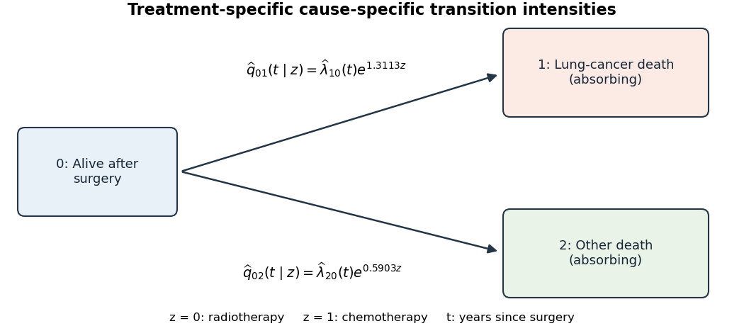
For treatment $z=0$ (radiotherapy) or $z=1$ (chemotherapy), define the transition intensityThe fitted Cox proportional-hazards models areHere ${\hat{\lambda }}_{10}$ and ${\hat{\lambda }}_{20}$ represent the estimated baseline cause-specific hazards for radiotherapy. More formally, the baseline estimates can be expressed as cumulative hazard measures with increments $d_k(t)/{\sum }_{i\in R(t)}{e}^{{\hat{\gamma }}_k{z}_i}$, rather than ordinary smooth functions. All outgoing intensities from states 1 and 2 vanish, and $q_{00}=-(q_{01}+q_{02})$. The treatment hazard ratios are 3.7111 and 1.8045 respectively. This model describes the two observed causes of death, not identifiable latent failure times after death has already occurred.

Among patients still alive at the same time after surgery, chemotherapy has an estimated lung-cancer death rate 3.71 times that of radiotherapy, assuming proportional cause-specific hazards. The estimated 95% confidence interval for this hazard ratio is $(1.583,8.697)$. Thus the fit suggests a higher instantaneous lung-cancer death rate on chemotherapy, with appreciable uncertainty in its size.

The null hypothesis of no treatment effect on that hazard is $H_0:{\gamma }_1=0$ against ${\gamma }_1\ne 0$. Its Wald test uses $Z=1.3113/0.4346\simeq 3.018$, approximately standard normal under the null hypothesis, with two-sided $p=0.00255$. This is evidence against equal lung-cancer death hazards in the fitted model. It is not a statement that five-year lung-cancer death probability is multiplied by 3.71 or that survival duration is divided by 3.71. The cumulative incidence function depends on both cause-specific hazards, and the model needs proportional-hazards and independent observation-censoring assumptions. In a randomised comparison the assigned treatment contrast is protected against baseline confounding, but the instantaneous comparison concerns the groups who have survived to the time in question; it does not identify a treatment effect within a common latent survivor subgroup.

The moment-based approach specifies marginal means, variances, and within-student covariances, without supplying a joint probability distribution for each count profile. It is a quasi-likelihood or generalized estimating equation strategy. The parameter interpreted as a structural-zero fraction is not automatically an actual probability of a structural-zero component merely because it appears in the moment formulas. A valid positive-definite working covariance and parameter identifiability must also be checked.

The printed covariance specification is not admissible for all the stated parameter values. For example, take $\pi =1/2$, $\tau =1$, and all three component means equal to 10. It gives diagonal variance 80 and off-diagonal covariance 100, so $\mathrm{Var}(Y_{i1}-Y_{i2})=80+80-2(100)=-40$. A covariance matrix cannot have a negative variance in any direction. Thus the moment approach requires additional admissibility restrictions or a valid working covariance; the parameter ranges alone do not define a valid model. This does not alter the hierarchical model, whose covariance derived below is positive semidefinite.

The alternative gives a full hierarchical mixture distribution, specifically a shared zero-inflated Gamma-Poisson count model: a common student random effect is zero with probability $\pi$, and otherwise has a Gamma distribution with mean 1 and variance $\tau$. Conditional on this effect, the three counts are independent Poisson random variables. Integrating it out induces both excess zeros and positive within-student dependence. Zero inflation is shared for the whole student, rather than independently reselected in each term. This full distribution supports likelihood-based inference but is more sensitive to the distributional assumptions.

The marginal mean in the hierarchical model has the same form as the proposed moment mean. Its marginal covariance does not, in general, equal the printed working covariance; the law of total covariance calculation below makes the distinction explicit. At $\tau =0$ the Gamma component is interpreted as its point-mass-at-one limit. At $\pi =1$ all counts are zero, and the log-mean parameterization and regression effects are not identifiable.

For the moment approach, write $m_i=\mathbb{E}{Y}_i$ and let $V_i$ be a positive-definite working covariance constructed from the proposed moment formulas. For identifiable mean coefficients $\theta$, let $D_i=\partial m_i/\partial {\theta }^T$. Generalized estimating equations take the formAcross independent students, correct mean specification and standard regularity conditions give consistent identifiable mean coefficients even if the working covariance is wrong. Sandwich covariance matrix standard errors useResidual second-moment estimating equations can estimate identifiable dispersion and association parameters. The marginal mean only identifies ${\gamma }_0={\beta }_0+\log (1-\pi )$, not ${\beta }_0$ and $\pi$ separately. Moment restrictions beyond the mean would be needed to separate them; as shown below, the printed restrictions do not generally recover the intended latent parameters.

For the hierarchical approach, maximize the observed-data likelihood after integrating out the random effect. Set ${\mu }_{ij}=e^{{\beta }_0+{\beta }^T{x}_i+{\alpha }_j}$, $r=1/\tau$, $M_i={\sum }_j{\mu }_{ij}$ and $s_i={\sum }_j{y}_{ij}$. The joint likelihood contribution isThe integral comes from multiplying three conditional Poisson mass functions by the Gamma density and integrating $b_i^{r+s_i-1}{e}^{-(r+M_i)b_i}$ over $b_i>0$. Independent students give $\ell ={\sum }_i\log L_i$. Direct numerical maximum likelihood or an expectation-maximization algorithm can be used; in an EM algorithm an all-zero profile has an uncertain latent component membership. Information-based likelihood standard errors apply under regular interior conditions, with special care for parameter boundaries.

With ${\alpha }_1=0$, the marginal moment model givesThus $e^{{\alpha }_2}$ and $e^{{\alpha }_3}$ are ratios of expected visits in Lent and Easter to expected visits in Michaelmas, respectively, at the same baseline covariates. These are population mean ratios, including students with no propensity to attend; they are not odds ratios or probabilities of any attendance.

In the hierarchical model, for a fixed positive student effect $b_i$, the conditional mean ratio is also $e^{{\alpha }_j}$. It describes a multiplicative within-student change in expected visits holding the student effect fixed. For the structural-zero component all three means are zero, so no nonzero ratio is defined there. Since the distribution of $b_i$ and the mixture weight do not vary by term, integrating out $b_i$ preserves this same marginal mean ratio. This is mean-ratio preservation under a multiplicative random effect: the conditional and marginal term coefficients coincide for this multiplicative log-link model. They need not coincide in a general nonlinear mixed model, such as a logistic random-effect model. A log-mean difference ${\alpha }_j$ is not a difference of expected logarithms of counts, which can be undefined at zero.

Keep baseline covariates fixed and put $q=1-\pi$, ${\mu }_j=e^{{\beta }_0+{\beta }^T{x}_i+{\alpha }_j}$, and $r=1/\tau$ for $\tau >0$. Integration of a Poisson count over the Gamma component givesThis negative binomial distribution has mean ${\mu }_j$ and variance ${\mu }_j+\tau {\mu }_j^2$. Therefore the unconditional one-term distribution is the zero-inflated negative binomial distributionIn particular its zero probability is $\pi +q(1+\tau {\mu }_j{)}^{-1/\tau }$, not simply $\pi$. As $\tau \downarrow 0$ this becomes a Zero-inflated Poisson distribution.

The mixing effect has $\mathbb{E}{b}_i=q$, $\mathbb{E}{b}_i^2=q(1+\tau )$ and $\mathrm{Var}(b_i)=q(\tau +\pi )$. The law of total variance and law of total covariance now giveEquivalently, for $\mu =({\mu }_1,{\mu }_2,{\mu }_3{)}^T$, $\mathbb{E}{Y}_i=q\mu$ and $\mathrm{Cov}(Y_i)=\mathrm{diag}(q\mu )+q(\tau +\pi )\mu {\mu }^T$. This also supplies raw second moments by adding $(\mathbb{E}{Y}_i)(\mathbb{E}{Y}_i{)}^T$. Dependence arises from both shared heterogeneity and shared structural zeros, even when the positive random effect is constant.

The printed moment variance matches the hierarchical variance at the same parameter values, but its printed off-diagonal covariance is $\tau {\mu }_j{\mu }_k$. Equality would require $\tau =q(\tau +\pi )$, or $\pi (\tau -q)=0$. It is therefore false to claim that the two approaches consistently estimate all the same parameters in general.

The precise distinction is between consistency of mean ratios and identification of structural parameters. In the hierarchical model, with $m_j=q{\mu }_j$, both the quadratic variance coefficient and the covariance coefficient in terms of the marginal mean areFor the moment parameterization, writing its parameters as ${\pi }_Q,{\tau }_Q,q_Q=1-{\pi }_Q$, these coefficients are $A_Q=({\pi }_Q+{\tau }_Q)/q_Q$ and $B_Q={\tau }_Q/q_Q^2$. Its intercept is identifiable from the mean only as ${\gamma }_{0Q}={\beta }_{0Q}+\log q_Q$. Matching the true first two moments demands $A_Q=B_Q=\kappa$. One solution always isFor $\kappa >1$ there is also a solution $q_Q=1/\kappa$, ${\pi }_Q=1-1/\kappa$, ${\tau }_Q=1/\kappa$, with the corresponding shifted intercept. Indeed eliminating ${\tau }_Q$ gives ${\pi }_Q({\tau }_Q-q_Q)=0$. This is moment aliasing in a shared zero-inflated count model: matching the moments does not identify the actual structural-zero probability.

For a concrete counterexample take $\pi =0.2,\tau =0.3$. Then $q=0.8$ and $\kappa =0.625$. The only admissible moment-matching choice is ${\pi }_Q=0,{\tau }_Q=0.625$, with an intercept shifted by $\log 0.8$; it cannot recover the true structural-zero proportion 0.2. Correct marginal means can give consistent term and baseline-covariate slopes with sandwich standard errors; they do not justify consistent estimation of the intended $\pi ,\tau$, or latent intercept. Nor does a mean-only estimating equation identify $\pi$ at all. Full-distribution inference provides information beyond these first two moments.

The likelihood-ratio statistic isThe null hypothesis $\pi =0$ is at the boundary of the permitted mixture weights. Assuming the remaining parameters are identifiable and interior, including $\tau >0$, an efficient normalized score for $\pi$ is asymptotically $Z\sim N(0,1)$ under the null hypothesis. The locally unconstrained quadratic log-likelihood maximizer is proportional to $Z$, while the constrained maximizer truncates it at zero. Thus $G^2\Rightarrow (\max (0,Z){)}^2$, giving the one-sided boundary likelihood-ratio limitHere ${\delta }_0$ is a point mass at zero. For a positive observed statistic the upper-tail probability is half the ordinary ${\chi }_1^2$ upper tail. The 5% critical value is the 90th percentile of ${\chi }_1^2$, about 2.7055, displayed as 2.71. Hence the reported likelihoods give a very marginal rejection of $\pi =0$ at 5%, with $p\simeq 0.04955$.

Using the ordinary 95th-percentile cutoff 3.84 would be inappropriate for this one-sided boundary test. The conclusion is close enough to the threshold that likelihood rounding matters: since each log-likelihood is printed to two decimals, the unrounded statistic can differ from 2.72 by nearly 0.02. The intended calculation rejects using the reported values, but an exact decision from the fitted data requires unrounded likelihoods. If the nuisance dispersion is also on its boundary or the mixture is not identifiable, the stated half-and-half null distribution needs reconsideration.