Past exam of the mathematics course of the University of Cambridge / 2012 / iii / Paper 73 / 2

Internal intermittency is the uneven distribution of activity within an already turbulent fluid: intense gradients and viscous dissipation occupy relatively small, fluctuating regions separated by much quieter regions. It concerns the internal field, rather than a turbulent/non-turbulent interface intermittently passing a probe.

Integral-scale intermittency is the variability of the energy-containing eddies and their local or time-dependent energy supply. Its modulation occurs on lengths and times of order $\ell$ and $\ell /u$, can depend strongly on forcing or initial conditions, and changes the background intensity experienced by smaller eddies.

Equilibrium-range intermittency concerns the increasing fluctuations of local transfer and viscous dissipation as the averaging scale is reduced below the integral scale of turbulence. It appears as non-Gaussian velocity-gradient statistics, fluctuating coarse-grained viscous dissipation and anomalous longitudinal structure function exponents. It includes the inertial range and its continuation into the dissipation range, where kinematic viscosity ultimately limits gradients. Large-scale modulation varies the local energy supply; small-scale intermittency concentrates and redistributes that supply. These effects can coexist, so they should not be identified simply because both broaden a distribution.

For the Landau intermittency counterexample, combine two locally homogeneous turbulent populations, with the same sufficiently wide inertial interval but different viscous dissipation rates ${ϵ}_1$ and ${ϵ}_2$. This can mean an ensemble randomly selected between two intensities, or large turbulent patches whose small-scale increments are sampled away from the patch boundaries. Suppose each population individually obeys the proposed universal coefficient ${\beta }_p$. If their proportions are $w$ and $1-w$, the combined longitudinal structure function isIts effective coefficient referenced to the global mean viscous dissipation is thereforeFor a concrete example let $w=1/2$ and ${ϵ}_{1,2}=ϵ(1\pm d)$, with $0<d<1$. ThenFor $p=6$ this is $1+d^2$, explicitly dependent on the strength of the large-scale modulation. For $p=2$ it is less than one by concavity. Thus coefficients based solely on mean viscous dissipation cannot be universal under arbitrary integral-scale intermittency. The common inertial interval can be maintained by taking both local Reynolds numbers sufficiently large.

At $p=3$ the ratio is exactly one. This exception is consistent with the signed third-order energy-flux law and must not be used to rescue universality of all other orders. For noninteger orders one uses absolute increments; the even-order examples already establish the counterexample without a sign convention ambiguity. The issue is the difference between a moment of the local viscous dissipation and the same power of its mean, not a failure of averaging itself.

Let ${ϵ}_{\mathrm{loc}}(\mathbf{x})=2\nu S_{ij}{S}_{ij}$ and define a coarse-grained energy dissipation at scale $r$, for example by a ball average,This is the random variable denoted ${ϵ}_{\mathrm{AV}}(r)$. The refined similarity hypothesis uses the local supply of energy available to motions of size $r$, rather than replacing it everywhere by a global mean. In its inertial range form,At high local Reynolds number, $V$ has a universal conditional distribution independent of ${ϵ}_r$, forcing details and $r$ within the inertial range. This givesFor signed odd orders the coefficients carry the appropriate sign; absolute moments use their own coefficients. Universality is retained in the normalized conditional velocity statistics, while the distribution of ${ϵ}_r$ can retain integral-scale information. This distinction resolves the particular averaging objection: its nonuniversal viscous dissipation moments are now explicitly present.

The quoted second viscous dissipation moment does not by itself determine every longitudinal structure function exponent. The extra lognormal intermittency model assumes $Y_r=\log ({ϵ}_r/ϵ)$ is Gaussian. Write its variance as ${\sigma }_r^2$. Normalization of the mean requires $⟨Y_r⟩=-{\sigma }_r^2/2$, soThe second-moment estimate gives $\exp ({\sigma }_r^2)=B(\ell /r{)}^{\mu }$. Hence, with $q=p/3$,In particular ${\zeta }_3=1$, ${\zeta }_2=2/3+\mu /9$ and ${\zeta }_6=2-\mu$.

The most problematic step is the extrapolation of a lognormal viscous dissipation law to rare events and all moment orders. It is not entailed by a measured second moment. Its quadratic exponents eventually decrease with $p$ and become negative for $p>3+6/\mu$. If the velocity has finite uniformly bounded moments, the bound $⟨|\Delta v{|}^p⟩\le 2^p⟨|u_x{|}^p⟩$ prohibits such divergence as $r\to 0$. Thus the model cannot be an unrestricted high-order inertial range law. This is a criticism of the lognormal closure, rather than an algebraic contradiction in refined similarity itself.

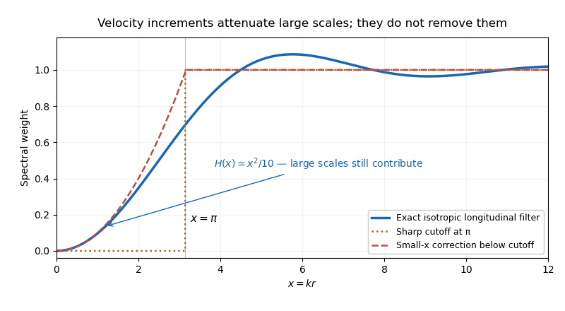
Write $S_2(r)=⟨(\Delta v{)}^2⟩$ and normalize the turbulent energy spectrum by ${\int }_0^{\infty }E(k)dk=⟨|\mathbf{u}{|}^2⟩/2$. In isotropic incompressible turbulence the longitudinal velocity correlation isCombining $S_2=2[Q_{LL}(0)-Q_{LL}(r)]$ with $Q_{LL}(0)=2\int Edk/3$ gives the exact spectral filterThe expression has a smooth removable limit at $x=0$. Its asymptotic forms areAn eddy much larger than $r$ contributes nearly the same velocity at the two points and mostly cancels in the increment. An eddy much smaller than $r$ contributes decorrelated velocities and does not cancel. Replacing the smooth transition of $H$ by a step at $kr=\pi$ therefore gives the common estimate $3S_2/4\simeq {\int }_{\pi /r}^{\infty }E(k)dk$. The cutoff corresponds roughly to a half wavelength equal to the point separation; its exact numerical location is conventional.

Keeping the leading nonzero low-wavenumber term gives the improved estimateIt remains imperfect because $kr$ is not small throughout the whole low-wavenumber interval and the exact kernel oscillates above the transition. The data sheet's alternative coefficient $1/{\pi }^2$ is a nearby approximate matching prescription; $1/10$ is the exact Taylor coefficient. Neither piecewise filter is an exact identity.

Higher-order longitudinal structure functions also retain large-scale information. Decompose $\mathbf{u}=\mathbf{U}+{\mathbf{u}}_s$, where $\mathbf{U}$ varies on a length much larger than $r$. Its longitudinal increment is $\Delta U_L\simeq r{\partial }_L{U}_L$, which is small but not zero. Expanding $(\Delta U_L+\Delta u_{s,L}{)}^p$ gives its own moments and mixed moments with the small-scale increment. Rare large gradients or correlated amplitude modulation can matter particularly strongly at large $p$.

Thus a velocity increment is not an exact scale-local bandpass filter. Its moments may retain large-scale strain and forcing information, undermining an unqualified claim of universal small-scale statistics determined by one local parameter. This observation alone does not refute an asymptotic inertial range theory: for a three-dimensional $k^{-5/3}$ spectrum, the low-wavenumber correction is mainly supplied by wavenumbers of order $1/r$, while an isolated integral-scale smooth contribution behaves as $r^2$ and is subleading to $r^{2/3}$. The issue is whether large-scale contamination and mixed moments actually become negligible in the regime and moment order being used.

Let the two-dimensional enstrophy cascade spectrum be $E(k)=C{k}^{-3}$ between $k_0$ and $k_d$, and choose a separation well inside the range: $k_0\ll k_c=\pi /r\ll k_d$. The high-wavenumber energy isThe low-wavenumber correction instead givesIts ratio to the preceding energy contribution is $({\pi }^2/4)\log (k_c/k_0)$, which is large when the separation is sufficiently far below the integral scale of turbulence. Consequentlyup to the stated piecewise-filter approximation and subleading contributions. Equivalently, if $Z_{<k_c}={\int }_0^{k_c}{k}^{2}E(k)dk$ is the cumulative enstrophy in motions larger than $r$, then $S_2\simeq r^2{Z}_{<k_c}/4$.

The leading increment variance is controlled by the accumulated enstrophy at scales larger than the separation, rather than the kinetic energy at smaller scales. For a $k^{-3}$ spectrum, each logarithmic wavenumber interval contributes the same amount to that enstrophy integral, so the conclusion does not mean that only the largest eddy supplies it. The logarithm is a marginal failure of a pure local $r^2$ estimate. The stipulated wide power-law range is essential, and the dominance need not hold at its upper spatial edge where $k_c/k_0$ is only of order one.