Past exam of the mathematics course of the University of Cambridge / 2012 / iii / Paper 73 (Turbulence)

Work with an incompressible Newtonian fluid of constant kinematic viscosity. The vorticity equation is $D\mathbf{\omega }/Dt=(\mathbf{\omega }\cdot \nabla )\mathbf{u}+\nu {\nabla }^2\mathbf{\omega }$. In the axisymmetric Burgers vortex the swirl does not advect the axial vorticity, and the stretching rate is ${\partial }_z{u}_z=\alpha$. Put $s(t)={\delta }^2(t)$ and $W={\omega }_z$. The Gaussian profile hasSubstitution into ${\partial }_{t}W+u_r{\partial }_{r}W=\alpha W+\nu {\nabla }^{2}W$ matches both the constant and $r^2$ terms precisely whenFor every finite positive initial $s_0$,The strain compresses the cross-section and stretches its vorticity, while kinematic viscosity spreads the core. The attracting radius is the balance of these effects; its relaxation time is ${\alpha }^{-1}$. Total circulation stays fixed because stretching increases the vorticity as the cross-sectional area decreases.

At the steady core radius, the swirl speed is of order ${\Gamma }_0/\delta$, and its velocity gradient tensor is of order ${\Gamma }_0/{\delta }^2$. Its viscous dissipation integrated over a cross-section therefore scales asThis is per unit length and per unit density. More precisely, for the swirl contribution, integration by parts relates the integrated strain viscous dissipation to $\nu \int W^{2}dA$; the boundary term vanishes for the $1/r$ swirl velocity. ThusMultiply by density for power per physical length. Here the azimuthal velocity's circulation $\Gamma$ is ${\Gamma }_0$, as follows by integrating $W$ over the cross-section. The result is finite as $\nu \to 0$ with strain and circulation held fixed. Local core viscous dissipation grows like ${\nu }^{-1}$ while its area shrinks like $\nu$. For ${\Gamma }_0/\nu \gg 1$, the swirl gradients dominate the background strain within the core.

This finite quantity is the excess viscous dissipation due to the vortex. The uniform straining flow alone dissipates $3\nu {\alpha }^2$ per unit volume, and integrating that over an infinite cross-section diverges. The total viscous dissipation of the complete idealized flow is therefore not a finite tube power unless the background is subtracted or spatially bounded.

A Burgers vortex sheet instead smooths a fixed velocity jump $U$ across a layer of thickness ${\delta }_s\sim \sqrt{\nu /\alpha }$. Its viscous dissipation per sheet area is of orderA tube with fixed circulation supports finite viscous dissipation in a vanishingly small core; a sheet with fixed velocity jump does not. This makes strained vortex tubes plausible intense dissipative structures at high Reynolds number. It does not assert that sheets are absent from turbulence: sheets can carry inertial range organization and become unstable, producing finer vortical structures.

For unforced incompressible flow, multiply the vorticity equation by ${\omega }_i$. The antisymmetric part of the velocity gradient tensor drops out of ${\omega }_i{\omega }_j{\partial }_j{u}_i$, leavingStatistical homogeneity removes mean divergences. Integration by parts, together with $\nabla \cdot \mathbf{\omega }=0$, givesThe last equality holds for the averages, not pointwise. It follows from the usual curl/divergence identity after the divergence terms have averaged to zero. Vortex stretching produces enstrophy, while viscous diffusion destroys it.

Let $T=\ell /u$, $ϵ\sim u^3/\ell$, and use the Kolmogorov microscales $\eta =({\nu }^3/ϵ{)}^{1/4}$ and ${\tau }_{\eta }=(\nu /ϵ{)}^{1/2}$. Since $⟨{\omega }^2⟩=ϵ/\nu$, a slowly changing mean enstrophy has a time derivative of order $ϵ/(\nu T)$. The usual small-scale estimate givesThe relative imbalance is consequently ${\tau }_{\eta }/T\sim (\nu /u\ell {)}^{1/2}={\mathrm{Re}}^{-1/2}$, yieldingThe estimate assumes an established high-Reynolds-number cascade and integral-time evolution of the mean, not a rapid initial transient. In a forced flow the exact balance includes $⟨\mathbf{\omega }\cdot \nabla \times \mathbf{f}⟩$; forcing smooth on the integral scale of turbulence is smaller than the leading small-scale terms.

Use $A=S+\Omega$, where $S$ is the rate-of-strain tensor and $\Omega$ is antisymmetric. For incompressible flow $\mathrm{tr}S=0$. Since ${\Omega }^2=(\mathbf{\omega }{\mathbf{\omega }}^T-{\omega }^{2}I)/4$, taking a trace givesThis uses the positive convention $R=\mathrm{tr}{A}^3/3$ specified here; a convention with the opposite sign for $R$ must not be mixed into the calculation. For a compressible flow there is an additional term $-3{\omega }^2\mathrm{tr}S/4$, so the displayed incompressible formula is not literally valid for every flow.

One can exhibit the required divergence directly. DefineDifferentiating, terms containing ${\partial }_i{u}_i$ vanish, and the two terms with a second derivative cancel after relabeling indices. Thereforein homogeneous turbulence with finite differentiable moments, or under periodic averaging. This is the Betchov relation. The preceding trace identity then impliesThe principal strain rates are the real eigenvalues of the symmetric matrix $S$. Incompressibility gives $a+b+c=0$, and the identity $a^3+b^3+c^3-3abc=(a+b+c)(a^2+b^2+c^2-ab-bc-ca)$ givesNo isotropy is required for this averaged tensor identity: statistical homogeneity and incompressibility are the key assumptions.

The high-Reynolds-number balance gives positive mean vortex stretching. The Betchov relation therefore gives $⟨abc⟩<0$. To connect this to a fixed longitudinal velocity derivative, additionally assume isotropic turbulence, or average over the direction of that derivative. For a unit vector $\mathbf{n}$, the derivative is $d={\mathbf{n}}^{T}S\mathbf{n}$. Uniform directional averaging, with $\mathrm{tr}S=0$, givesFor example these identities follow by averaging products of direction cosines on a sphere. Hence in isotropic turbulenceand division by the positive derivative variance to the power $3/2$ gives negative longitudinal velocity-gradient skewness. Homogeneity alone does not fix the orientation statistics and does not establish this sign for every chosen coordinate direction.

Order the principal strain rates as $a\ge b\ge c$. Except at degeneracies, $a>0$ and $c<0$, so $abc<0$ corresponds to $b>0$: two extensional directions and one compressive direction, or bi-axial strain. The negative average of $abc$ says that such configurations dominate this cubic amplitude-weighted statistic over axial-extension configurations with $b<0$. In the usual physical interpretation, comparably intense strain events are therefore biased toward bi-axial extension.

An unweighted frequency claim needs more information. As a counterexample to deducing it solely from the cubic average, assign strain eigenvalues $(1,1,-2)$ to 10% of samples and $(-0.1,-0.1,0.2)$ to 90%, with randomly oriented eigenvectors. Then $⟨abc⟩=-0.1982<0$, despite bi-axial extension occurring in only 10% of the samples. This example addresses what the moment inequality can infer, not a construction of a complete turbulent velocity field. A measured frequency preference is a further statistical observation.

The geometric significance is that a fluid element stretches in two directions and contracts in the third, becoming sheet-like while preserving volume. Distributed vorticity is swept into thin layers and its component along an extensional direction is amplified. The associated shear layers can subsequently roll up and produce vortex tubes. Thus the weighted strain bias helps explain sheet formation in the energy cascade even though the most intense dissipative structures can be tubes.

In the Townsend-Betchov cascade cartoon, bi-axial strain sweeps distributed vorticity into extended sheets at the upper part of the inertial range. These are predominantly inviscid structures: their shape and instability arise from advection and strain rather than local viscous smoothing. Strong velocity variation across a thin sheet permits Kelvin-Helmholtz instability, roll-up and three-dimensional deformation. The resulting small vortex tubes are stretched into still finer cores.

At the dissipative end, stretching and kinematic viscosity balance in Burgers-like cores. A core of strain rate $s$ has radius of order $(\nu /s{)}^{1/2}$; taking $s\sim (ϵ/\nu {)}^{1/2}$ gives the Kolmogorov length $({\nu }^3/ϵ{)}^{1/4}$. Circulation and shrinking cross-section allow finite integrated tube viscous dissipation. Thus sheet formation and tube formation play different roles, rather than the entire cascade being a succession of identical geometrical eddies.

The cartoon challenges a literal, uniformly self-similar, step-by-step cascade with independent interactions only between neighboring scales. Large-scale sheet formation can generate much smaller scales through an instability, and the resulting structures retain coherent spatial organization. A branching model that assumes every scale-transfer step has the same geometry and loses information about the parent flow can miss this mechanism. Closures that erase the relevant phase correlations also have difficulty representing its concentrated gradients and intermittency. The objection is to these dynamical assumptions, not to conservation of energy or the existence of a mean energy flux through scales. The cartoon alone is not a proof that all spectral transfer is nonlocal.

Internal intermittency is the uneven distribution of activity within an already turbulent fluid: intense gradients and viscous dissipation occupy relatively small, fluctuating regions separated by much quieter regions. It concerns the internal field, rather than a turbulent/non-turbulent interface intermittently passing a probe.

Integral-scale intermittency is the variability of the energy-containing eddies and their local or time-dependent energy supply. Its modulation occurs on lengths and times of order $\ell$ and $\ell /u$, can depend strongly on forcing or initial conditions, and changes the background intensity experienced by smaller eddies.

Equilibrium-range intermittency concerns the increasing fluctuations of local transfer and viscous dissipation as the averaging scale is reduced below the integral scale of turbulence. It appears as non-Gaussian velocity-gradient statistics, fluctuating coarse-grained viscous dissipation and anomalous longitudinal structure function exponents. It includes the inertial range and its continuation into the dissipation range, where kinematic viscosity ultimately limits gradients. Large-scale modulation varies the local energy supply; small-scale intermittency concentrates and redistributes that supply. These effects can coexist, so they should not be identified simply because both broaden a distribution.

For the Landau intermittency counterexample, combine two locally homogeneous turbulent populations, with the same sufficiently wide inertial interval but different viscous dissipation rates ${ϵ}_1$ and ${ϵ}_2$. This can mean an ensemble randomly selected between two intensities, or large turbulent patches whose small-scale increments are sampled away from the patch boundaries. Suppose each population individually obeys the proposed universal coefficient ${\beta }_p$. If their proportions are $w$ and $1-w$, the combined longitudinal structure function isIts effective coefficient referenced to the global mean viscous dissipation is thereforeFor a concrete example let $w=1/2$ and ${ϵ}_{1,2}=ϵ(1\pm d)$, with $0<d<1$. ThenFor $p=6$ this is $1+d^2$, explicitly dependent on the strength of the large-scale modulation. For $p=2$ it is less than one by concavity. Thus coefficients based solely on mean viscous dissipation cannot be universal under arbitrary integral-scale intermittency. The common inertial interval can be maintained by taking both local Reynolds numbers sufficiently large.

At $p=3$ the ratio is exactly one. This exception is consistent with the signed third-order energy-flux law and must not be used to rescue universality of all other orders. For noninteger orders one uses absolute increments; the even-order examples already establish the counterexample without a sign convention ambiguity. The issue is the difference between a moment of the local viscous dissipation and the same power of its mean, not a failure of averaging itself.

Let ${ϵ}_{\mathrm{loc}}(\mathbf{x})=2\nu S_{ij}{S}_{ij}$ and define a coarse-grained energy dissipation at scale $r$, for example by a ball average,This is the random variable denoted ${ϵ}_{\mathrm{AV}}(r)$. The refined similarity hypothesis uses the local supply of energy available to motions of size $r$, rather than replacing it everywhere by a global mean. In its inertial range form,At high local Reynolds number, $V$ has a universal conditional distribution independent of ${ϵ}_r$, forcing details and $r$ within the inertial range. This givesFor signed odd orders the coefficients carry the appropriate sign; absolute moments use their own coefficients. Universality is retained in the normalized conditional velocity statistics, while the distribution of ${ϵ}_r$ can retain integral-scale information. This distinction resolves the particular averaging objection: its nonuniversal viscous dissipation moments are now explicitly present.

The quoted second viscous dissipation moment does not by itself determine every longitudinal structure function exponent. The extra lognormal intermittency model assumes $Y_r=\log ({ϵ}_r/ϵ)$ is Gaussian. Write its variance as ${\sigma }_r^2$. Normalization of the mean requires $⟨Y_r⟩=-{\sigma }_r^2/2$, soThe second-moment estimate gives $\exp ({\sigma }_r^2)=B(\ell /r{)}^{\mu }$. Hence, with $q=p/3$,In particular ${\zeta }_3=1$, ${\zeta }_2=2/3+\mu /9$ and ${\zeta }_6=2-\mu$.

The most problematic step is the extrapolation of a lognormal viscous dissipation law to rare events and all moment orders. It is not entailed by a measured second moment. Its quadratic exponents eventually decrease with $p$ and become negative for $p>3+6/\mu$. If the velocity has finite uniformly bounded moments, the bound $⟨|\Delta v{|}^p⟩\le 2^p⟨|u_x{|}^p⟩$ prohibits such divergence as $r\to 0$. Thus the model cannot be an unrestricted high-order inertial range law. This is a criticism of the lognormal closure, rather than an algebraic contradiction in refined similarity itself.

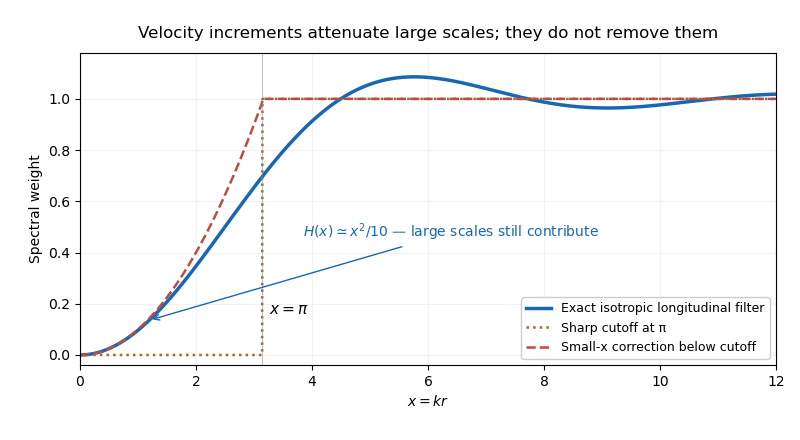
Write $S_2(r)=⟨(\Delta v{)}^2⟩$ and normalize the turbulent energy spectrum by ${\int }_0^{\infty }E(k)dk=⟨|\mathbf{u}{|}^2⟩/2$. In isotropic incompressible turbulence the longitudinal velocity correlation isCombining $S_2=2[Q_{LL}(0)-Q_{LL}(r)]$ with $Q_{LL}(0)=2\int Edk/3$ gives the exact spectral filterThe expression has a smooth removable limit at $x=0$. Its asymptotic forms areAn eddy much larger than $r$ contributes nearly the same velocity at the two points and mostly cancels in the increment. An eddy much smaller than $r$ contributes decorrelated velocities and does not cancel. Replacing the smooth transition of $H$ by a step at $kr=\pi$ therefore gives the common estimate $3S_2/4\simeq {\int }_{\pi /r}^{\infty }E(k)dk$. The cutoff corresponds roughly to a half wavelength equal to the point separation; its exact numerical location is conventional.

Keeping the leading nonzero low-wavenumber term gives the improved estimateIt remains imperfect because $kr$ is not small throughout the whole low-wavenumber interval and the exact kernel oscillates above the transition. The data sheet's alternative coefficient $1/{\pi }^2$ is a nearby approximate matching prescription; $1/10$ is the exact Taylor coefficient. Neither piecewise filter is an exact identity.

Higher-order longitudinal structure functions also retain large-scale information. Decompose $\mathbf{u}=\mathbf{U}+{\mathbf{u}}_s$, where $\mathbf{U}$ varies on a length much larger than $r$. Its longitudinal increment is $\Delta U_L\simeq r{\partial }_L{U}_L$, which is small but not zero. Expanding $(\Delta U_L+\Delta u_{s,L}{)}^p$ gives its own moments and mixed moments with the small-scale increment. Rare large gradients or correlated amplitude modulation can matter particularly strongly at large $p$.

Thus a velocity increment is not an exact scale-local bandpass filter. Its moments may retain large-scale strain and forcing information, undermining an unqualified claim of universal small-scale statistics determined by one local parameter. This observation alone does not refute an asymptotic inertial range theory: for a three-dimensional $k^{-5/3}$ spectrum, the low-wavenumber correction is mainly supplied by wavenumbers of order $1/r$, while an isolated integral-scale smooth contribution behaves as $r^2$ and is subleading to $r^{2/3}$. The issue is whether large-scale contamination and mixed moments actually become negligible in the regime and moment order being used.

Let the two-dimensional enstrophy cascade spectrum be $E(k)=C{k}^{-3}$ between $k_0$ and $k_d$, and choose a separation well inside the range: $k_0\ll k_c=\pi /r\ll k_d$. The high-wavenumber energy isThe low-wavenumber correction instead givesIts ratio to the preceding energy contribution is $({\pi }^2/4)\log (k_c/k_0)$, which is large when the separation is sufficiently far below the integral scale of turbulence. Consequentlyup to the stated piecewise-filter approximation and subleading contributions. Equivalently, if $Z_{<k_c}={\int }_0^{k_c}{k}^{2}E(k)dk$ is the cumulative enstrophy in motions larger than $r$, then $S_2\simeq r^2{Z}_{<k_c}/4$.

The leading increment variance is controlled by the accumulated enstrophy at scales larger than the separation, rather than the kinetic energy at smaller scales. For a $k^{-3}$ spectrum, each logarithmic wavenumber interval contributes the same amount to that enstrophy integral, so the conclusion does not mean that only the largest eddy supplies it. The logarithm is a marginal failure of a pure local $r^2$ estimate. The stipulated wide power-law range is essential, and the dominance need not hold at its upper spatial edge where $k_c/k_0$ is only of order one.

Consider an unforced incompressible flow with localized vorticity and sufficient smoothness for integration by parts. Define the hydrodynamic impulse per unit density by $\mathbf{I}=\frac{1}{2}\int \mathbf{x}\times \mathbf{\omega }dV$, denoting the vector impulse by $\mathbf{I}$ to distinguish it from the later scalar $L$. The vorticity equation can be writtenThe supplied identity, integrated over all space, gives $\frac{1}{2}\int \mathbf{x}\times \nabla \times \mathbf{F}dV=\int \mathbf{F}dV$, because $\mathbf{F}$ is localized and its surface terms vanish. ThereforeThe second integral is a vanishing surface integral. The vector identity $\mathbf{u}\times \mathbf{\omega }=\nabla (|\mathbf{u}{|}^2/2)-(\mathbf{u}\cdot \nabla )\mathbf{u}$ and incompressibility reduce the first to surface terms proportional to the quadratic velocity. Those vanish for $\mathbf{u}=O(R^{-3})$. Thus

For a large spherical control volume define ${\mathbf{P}}_R={\int }_{V_R}\mathbf{u}dV$. The impulse relation is $\mathbf{I}=(3/2){\lim }_{R\to \infty }{\mathbf{P}}_R$ for this localized field. The factor is important: impulse is not simply the integral of velocity, since an $R^{-3}$ velocity tail has a nonvanishing contribution in the impulse integration by parts involving a factor of $R$.

Using pressure per unit density $\Pi$ and the Navier-Stokes equation givesThe advective flux is $O(R^{-4})$, the pressure force is $O(R^{-1})$, and the viscous term is $O(\nu R^{-2})$ under the regular far-field derivative decay. All vanish as $R\to \infty$. The localized eddy cannot change its total impulse without a net external momentum input. Pressure redistributes momentum internally but its resultant force on an increasingly distant control surface tends to zero. At finite $R$, boundary forces need not vanish exactly; the all-space limit is the invariant statement.

Let $C(r)=⟨\mathbf{u}(\mathbf{x})\cdot \mathbf{u}(\mathbf{x}+\mathbf{r})⟩$ in zero-mean isotropic turbulence. Define the scalar Saffman integral $L={\int }_{{\mathbb{R}}^3}C(r)d^{3}r=4\pi {\int }_0^{\infty }{r}^{2}C(r)dr$. The spectral transform isFor an integrable $r^{2}C(r)$, dominated convergence applied to $\sin (kr)/(kr)$ givesA further $O(k^4)$ expansion requires an additional correlation moment and is not automatic from finite $L$. The normalization agrees with $\int Edk=⟨|\mathbf{u}{|}^2⟩/2$.

For a control volume $V$ put ${\mathbf{P}}_V={\int }_V\mathbf{u}dV$. Statistical homogeneity gives the exact finite-volume identityFor geometrically similar volumes increasing without bound, the overlap fraction $|V\cap (V-\mathbf{r})|/|V|$ tends to one at every fixed separation. If $C$ is absolutely integrable, dominated convergence givesThe printed finite-large-volume expression is the corresponding asymptotic approximation, not an exact identity for an arbitrary finite volume. For instance, positive nonzero $C$ with a finite correlation length gives an overlap fraction smaller than one and hence a strictly smaller finite-volume value. The limit also shows $L\ge 0$; a nonzero Saffman integral is positive.

A large spherical region contains $N\sim V_R/{\ell }^3$ energy-containing eddies. If their hydrodynamic impulses have zero mean, finite variance and sufficiently short-range correlations, the mean-square sum grows as $N$, rather than $N^2$. In the ideal independent case,The spherical impulse-momentum relation makes the integrated velocity proportional to this sum for isolated enclosed structures. In a full field, external dipolar velocities and boundary effects can change the coefficient; they do not alter the volume scaling under these random-impulse statistics. ThusIt is a random walk law for momentum fluctuations, not an extensive mean flow. Although the mean impulse is zero by isotropy, its variance need not vanish. The Saffman integral measures this large-volume momentum-fluctuation density. If every eddy had exactly zero impulse or correlations enforced systematic cancellation, this leading density could vanish and a different small-wavenumber spectrum could result.

Write $u^2=⟨u_x^2⟩$ for the one-component variance and $Q_{LL}=u^{2}f(r)$. Isotropy gives $Q_{ij}=u^2[(f-g)n_i{n}_j+g{\delta }_{ij}]$, and incompressibility gives $g=f+r{f}^{\prime }/2$. Taking the trace yieldsTherefore, with a regular correlation at the origin,For $L>0$, the longitudinal velocity correlation has the tail $u^{2}f(r)\sim L/(4\pi r^3)$. Its physical source is the velocity induced far from a localized eddy with nonzero hydrodynamic impulse. The hydrodynamic Biot-Savart kernel gives the dipolar far fieldThe absence of a vorticity monopole and the surviving impulse dipole give the $r^{-3}$ power. Random eddy impulses thus produce long-range velocity correlations despite the vorticity itself being concentrated in localized structures. Incompressibility also explains how a distant pressure response can redistribute velocity without transporting local vorticity there.

There is no inconsistency with integrability of the trace correlation. At leading order, $g\sim -f/2$, soThe longitudinal and transverse dipolar tails cancel in the trace. The scalar Saffman integral can remain finite even though individual tensor components have long-range, direction-dependent tails.

Multiply the Kármán-Howarth equation for $C(r,t)$ by $4\pi r^2$ and integrate in $r$. Integration by parts gives the exact boundary-flux expressionAt the origin smooth isotropic correlations give $K=O(r)$ or smaller and $C^{\prime }=O(r)$, so both boundary terms vanish. At infinity the usual regular power-law decay $K=O(r^{-4})$, with the corresponding derivative decay, makes the first term tend to zero. A sufficiently smooth integrable trace correlation makes $r^2{C}^{\prime }\to 0$ as well. Under these physical far-field conditions,The exact required conditions are the limits of these two boundary fluxes. A bare big-$O$ condition on $K$ without control of its derivatives is not by itself a rigorous sufficient condition: the smooth tail $K(r)=r^{-4}\sin (r^2)$ is $O(r^{-4})$, but $r^{-1}(r^{4}K{)}^{\prime }=2\cos (r^2)$ has no zero limit. The intended power-law assumption excludes such increasingly rapid far-field oscillations; this qualification is needed in a literal proof.

Physically, $L$ is the large-volume momentum variance divided by volume. Internal advective and pressure forces exchange momentum among eddies but do not provide a net impulse to the whole unforced field. For a large spherical region, the variance balance is driven by its boundary momentum flux. The stated correlation decay makes that contribution negligible per unit volume as the region grows. Thus the conservation law preserves momentum-fluctuation density, not kinetic energy. kinematic viscosity can remove kinetic energy while leaving this integral invariant.

Let $\mathcal{E}=⟨|\mathbf{u}{|}^2⟩/2$ be the turbulent kinetic energy per unit mass. In addition to $L>0$ and high Reynolds number, use the usual self-preserving large-eddy decay assumption: the normalized large-scale correlation has a fixed shape, sowhere $C_L>0$ is constant. For freely decaying high-Reynolds-number turbulence, the cascade viscous dissipation law is $ϵ=C_{ϵ}{\mathcal{E}}^{3/2}/\ell$. The kinetic-energy balance therefore givesPut $A=C_{ϵ}{C}_L^{1/3}{L}^{-1/3}$. Integrating,The constant $t_{\ast }$ is a virtual time origin. This is the Saffman decay law. The energy decreases while the integral scale of turbulence grows so that the conserved large-volume momentum variance remains constant.

The exponent does not follow from the invariant alone: it also uses unforced decay, one evolving large-eddy length and an asymptotically constant cascade viscous dissipation coefficient. A changing normalized spectral shape or a confining boundary can invalidate that closure. Moreover $\mathrm{Re}\sim {\mathcal{E}}^{1/2}\ell /\nu \propto (t-t_{\ast }{)}^{-1/5}$, so at fixed kinematic viscosity the high-Reynolds-number decay regime eventually ends; the $-6/5$ law is not a claim about the ultimate viscous limit.