Synchronous radius and its limits. Kepler's third law for a circumplanetary orbit givesHere is the gravitational constant. A planet-synchronous orbit repeats after one spin period. A planet-stationary orbit additionally requires a circular orbit, zero orbital inclination to the equator and prograde motion. Then an antenna fixed on the ground points continuously at the same satellite; merely matching the orbital period does not give this property.
Write the planetary radius as . Requiring the semi-major axis to exceed gives . The stellar tidal force restricts the circumplanetary orbit to the Hill sphere, of radius . ThusThese are the surface and Hill-radius constraints in the idealized spherical, small- model. Long-term prograde stability generally requires a radius appreciably inside the Hill sphere; for nonzero orbital eccentricity, the surface constraint applies to the periapsis, not just to the semi-major axis.
Collision time and the launch population. A phase-mixed isotropic swarm occupies a shell of radial scale . Its number density scales as , its relative speed as , and its geometric collision cross-section as . Consequently the total collision rate scales as . To give the numerical normalization used here, adopt an effective shell volume . At a fixed position the velocity directions are uniformly distributed in the tangent plane, so their mean relative speed is . For an unordered pair, the collision cross-section is , givingThus the mean interval between collisions is in this large-population kinetic model. The effective shell width fixes an order-one coefficient: small orbital eccentricity and random planes alone do not specify a unique radial probability density. Phase mixing, negligible gravitational focusing, , and uncorrelated encounters are implicit in this estimate. Exactly identical orbital periods with perfectly fixed phases do not themselves produce a memoryless collision process.
For nearly planet-stationary orbits with , the swarm volume is smaller by a factor of order , while the relative speed is smaller by the same factor, since vertical motion of scale dominates the eccentric motion. The two changes cancel in the rate : there is no parametric factor in the collision time within the same phase-mixed kinetic approximation. Numerical factors and phase correlations can differ. This is not an argument that bringing all satellites into one nearly circular plane makes their phases random.
With , an Inhomogeneous Poisson process has cumulative hazard functionThe survival function of the first collision is . Setting the expected number of collisions to one givesThis is a characteristic first-event population, with probability of an earlier event. It is not a median: the median has an additional factor .
Which population collides next? Immediately after the first disruption let and . The latter follows from mass conservation for equal-density spherical pieces. Using the same unordered-pair counting and geometric collision cross-sections as above, define ; thenHere stand for the usual large-population approximations to . The factor two distinguishing identical and different species is essential. The probability that the next collision is fragment–fragment isIt is the most likely type if and . It has probability greater than one half ifFor , a strongly fragment-dominated next event therefore requires ; the fragment–satellite comparison is more restrictive than the satellite–satellite comparison. If , the next event must be fragment–fragment, provided fragments remain.
Population equations and the normalization discrepancy. Every satellite–satellite event produces fragments and destroys two satellites. Every satellite–fragment event produces a net fragments and destroys one satellite; every fragment–fragment event destroys two fragments. Consistent collision counting therefore givesFor , and . The last two terms in are then twice those in the printed equation. This is a genuine factor-of-two inconsistency: equal-size fragment pairs have a collision cross-section smaller by , so their event rate must be if the satellite event rate is ; destroying both fragments necessarily gives the sink .
If the printed equation is taken as a prescribed approximate rate model instead, its implicit event rates are , and . Under precisely that mixed normalization, its corresponding satellite equation isThe printed source term also neglects the consumed fragment in a satellite–fragment event, a legitimate relative approximation. That approximation does not repair the pair-counting discrepancy.
The ensuing cascade. This is a two-size fragmentation cascade. First use the printed approximate model, dropping satellite–satellite events as requested. Put , , and take . ThenIntegrating this linear differential equation, with and , givesInitially the collisional cascade grows if , with approximate early exponential growth time when the satellite population is nearly fixed. The fragment population reaches its maximum atAfterwards satellites are depleted and fragment–fragment losses dominate. For the continuum solution has , , withWhen no satellites remain initially, directly. Small integer populations eventually invalidate these deterministic differential equations.
The consistently counted model has, to leading order in , exactly the same curve and peak, but both retained time derivatives are twice as large. Its growth time is , and . Keeping and the consumed fragment replaces by and in the curve by . This explicitly separates the physical collision bookkeeping from the printed normalization while giving the evolution under both conventions.
Specific orbital energy, orbital eccentricity and the distribution. Let , and . Choose positive to mean an outward radial kick. At release the tangential and radial velocities are and . The specific orbital energy and specific angular momentum areUsing and therefore givesThe denominator must be positive for an elliptic Kepler orbit. A vanishing denominator describes a parabolic Kepler orbit; negative is the signed semi-major axis of a hyperbolic Kepler orbit.
Differentiating the squared orbital eccentricity givesIn the small-kick regime , . Thus the minimum is at , withThe entire expression, including the term, lies under the square root in the PDF. This minimum is not a universal statement for arbitrary kick size. For example , reverses the circular velocity and gives a retrograde circular orbit with ; the displayed stationary value is then not the global minimum.
For , every kick direction gives a bound prograde Kepler orbit. The two endpoint maxima, one at each end of the accessible curve, areThe positive endpoint is the global maximum. There is one interior minimum, at the location just found. Uniform gives the kick-orbit distributionBoth signs of the radial kick occupy the same – curve; they have opposite apsidal orientations. The distribution is concentrated near its endpoints, with integrable square-root singularities. For larger kicks retain the parametric curve and its bound portion ; an unbound branch begins at , . In particular, a sketch of a wholly elliptic population presupposes the bound-kick restriction above.
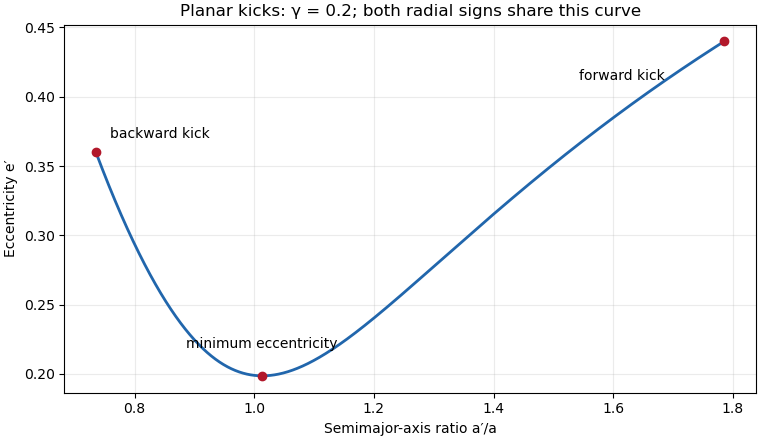
Eccentricity and semimajor-axis distribution for isotropic planar velocity kicks of magnitude 0.2 times the circular speed
. Details. The eccentricity vector at release has radial component and tangential component . With the release radius chosen as zero longitude,This also directly verifies the squared orbital eccentricity above and fixes the sign convention for the longitude of periapsis.
The 1:1 encounter window. Exact equality of orbital periods requires , hence . There are two kick directions with this cosine when . To quantify a finite window one must specify a return time: near exact commensurability, consider the particle's first complete return to its release point. During that time the source advances through . Its longitudinal miss distance is, to first order,Thus gives the two-sided cosine windowIntegrating over that window gives, to leading order for a narrow window away from ,The printed fraction is half this value. It is obtained by retaining only one side of the semi-major axis window, or only one of the two kick-angle branches. Neither restriction is in the question. Thus the printed coefficient cannot be shown for the stated uniform population and a symmetric first-return distance criterion. This already exhibits the discrepancy under the usual longitudinal approximation; minimizing the distance over the encounter interval introduces a further velocity-direction correction, not a missing branch. With arbitrarily long observation times, noncommensurate bound trajectories can also return arbitrarily close to the common release point, so an eventual-encounter fraction is a different, time-dependent question.
Rotating-frame sketches. In the rotating reference frame of the source put radially outward, along the source's motion and , where . The linear Hill equations for a stellar Kepler orbit, with initial displacement zero, give the velocity-kick epicycleThese solve , and reproduce the initial kick. For , the particle starts forward, moves outward and drifts backward; the curve has a loop each orbital cycle, with net per cycle. For , both coordinates reverse: it moves inward and drifts forward by . For , the leading trajectory is a closed epicyclic ellipse,It starts at the top of the ellipse moving radially outward and returns to the source after one period to this order. Its exact semi-major axis differs from at order , so exact closure is not implied. The local sketches require , in particular for the drifting cases.
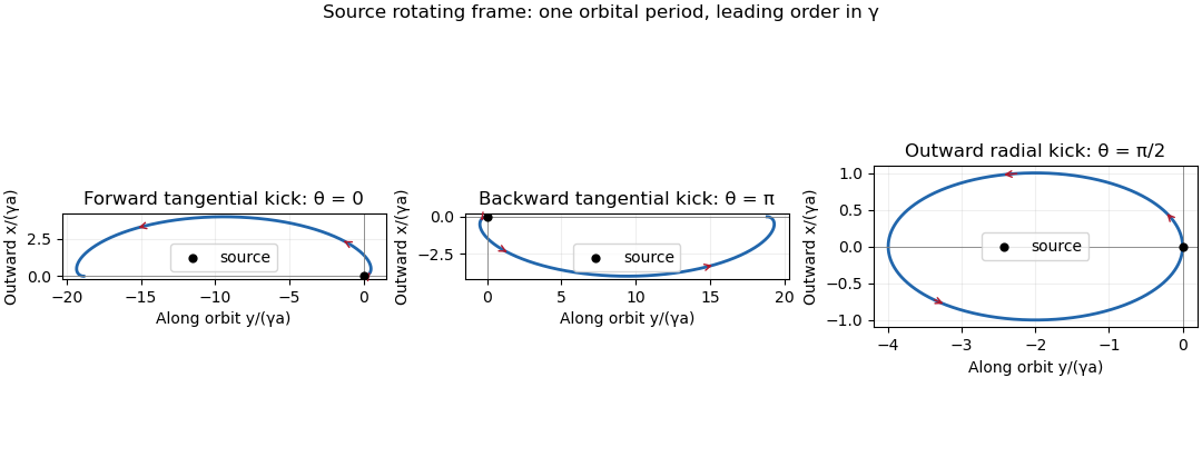
Particle trajectories after tangential prograde, tangential retrograde and outward radial kicks in the source rotating frame
. Details. Validity and the complete angular equation. The Lagrange planetary equations here describe a planar, circular-planet, small-orbital eccentricity, weakly perturbed exterior mean-motion resonance. Require , , one isolated slowly varying resonant argument, perturbation times long compared with an orbital period, and no close planetary encounters. Other resonant harmonics and short-period terms must be negligible; coefficients may be frozen only across a narrow range of semi-major axis. Take , or in a reduced integer ratio. Exactly makes the longitude of periapsis undefined, so the displayed angular variables must then be replaced by nonsingular eccentricity vector components.
Neglecting the perturbation to the accumulated mean longitude gives ; this is an accumulated-phase approximation, not differentiation of a fictitious expression while discarding . With ,Differentiating, using and the supplied orbital element equations, gives the full result within this constant-coefficient model:An equivalent formula replaces the last two terms in brackets by . No derivatives of are included because they were specified as constants.
A full fixed point requires and . Hence or , with its corresponding detuned semi-major axis fixed byAt either point . The longitude of periapsis still precesses, so the fixed point refers to the reduced resonant dynamics.
Linear stability analysis and encounter geometry. Linearizing the full equation about a fixed point givesFor , is a center equilibrium and zero is a saddle equilibrium. For , is always a center equilibrium, while zero is a saddle equilibrium ifAt sufficiently small orbital eccentricity the full truncated equations instead admit a center at zero as well; equality is a degenerate case requiring higher-order analysis. Thus an unconditional instability claim at zero does not follow from the full equation. In the usual fixed-eccentricity weak-resonance regime the inequality holds and the stable libration center is for either order.
The physical explanation is resonance protection. At equal mean longitudes, the conjunction direction relative to periapsis obeys modulo . For , places conjunction near periapsis, where the exterior particle comes closest to the planet; places it near apoapsis. For , zero includes both apsidal conjunctions, one of them near periapsis, whereas places the two conjunction branches near quadrature. The protected arrangements give restoring kicks in the positive- leading-harmonic model. This geometric explanation is conditional on its non-crossing, small-orbital eccentricity approximation; it does not override the low- term retained in the full stability calculation.
Small resonant-argument librations. Define the nominal resonant semi-major axis and the displaced center byThis follows by expanding and taking . It gives the requested initial semi-major axis to first order in the precession-induced detuning; and .
For the pendulum approximation of a mean-motion resonance, also require fractional changes in small across a libration, and precession terms small compared with . In particular for makes the extra full-equation curvature negligible; for , small fractional eccentricity changes require . Freeze in the leading restoring coefficient and setThen obeys simple harmonic motion. Using , and integrating the remaining Lagrange planetary equations givesThe omitted apsidal modulation comes from higher perturbative orders and . All expressions are leading resonant approximations, valid while the omitted fractional changes remain small. The small-libration phase portrait iswith period . The semi-major axis half-width is and the orbital eccentricity half-width is .
Dividing the original and equations gives the exact invariant of their retained terms,Thus the – plot is a segment of this increasing curve traversed back and forth, not a closed ellipse. Locally its slope is .
Finite amplitude and the separatrix. Keep the same weak-resonance approximation but allow to be finite. The leading angular equation is , or . Multiplication by givesThis resonant pendulum energy is constant in the pendulum approximation of a mean-motion resonance. It is not an exact integral of the earlier full equation when and its restoring coefficient vary: the term alone prevents that conclusion in general.
For the phase portrait has closed libration curves around , withwhere is the complete elliptic integral of the first kind. The largest speed is and the leading semi-major axis half-width is . As , the energy approaches , the separatrix through the saddles at zero and ; the particle spends increasingly long intervals near those saddles. With ,At exactly , , the particle stays at the unstable fixed point in the ideal model. Nonstationary separatrix trajectories approach the saddle only in infinite time; above separatrix energy, the resonant argument circulates and resonance protection is lost. These distinctions matter when describing the limiting motion.
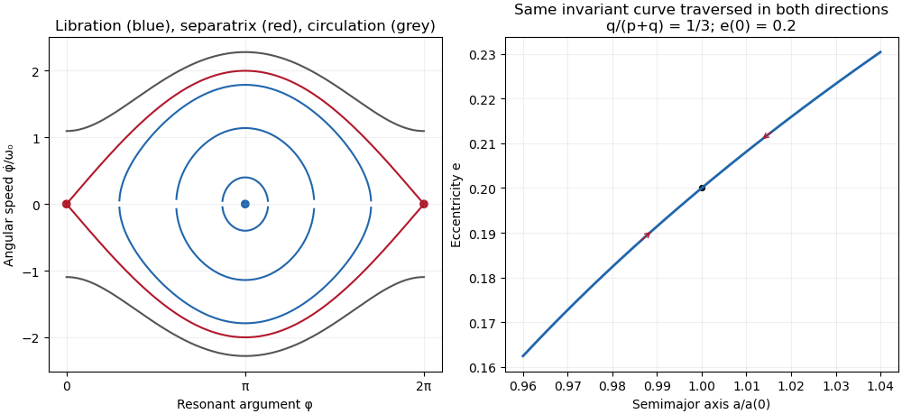
Resonant pendulum libration curves, separatrix and circulation, with the eccentricity versus semimajor-axis invariant
. Details. Eigenfrequencies and mode geometry. Write and . The characteristic polynomial is . Therefore the two distinct real eigenvalues areThe sign assumptions imply and ; they do not alone imply . A positive lower frequency additionally requires , as in the usual nondegenerate physical Laplace-Lagrange secular matrix.
Distinct eigenvalues give an eigenbasis, and each secular eigenmode evolves by multiplication by . Hencewith nonnegative amplitudes and initial phases. The second row of each eigenvalue equation gives . For the upper eigenvalue this ratio is negative, whereas for the lower one it is positive. ThusThe upper secular eigenmode has anti-aligned apsides, and the lower has aligned apsides. If one amplitude vanishes, its phase is immaterial.
The initial vector sums. The planet-1 modal vectors point at and . Their resultant at requires . The planet-2 vectors point at and ; their resultant at requires . These follow by resolving components perpendicular to each resultant. In particular the specified phases constrain the matrix: . They cannot be imposed on an arbitrary matrix satisfying only the sign assumptions.
Put and let . For a matrix compatible with those phases,At zero the resultants have lengths and and precisely the specified longitudes of periapsis. The diagram uses , as a drawing normalization, not as an additional assumption on the physical planets.


Each modal vector rotates counterclockwise if its eigenvalue is positive; their sum executes a beat at frequency . For these phases,The orbital eccentricities exchange their maxima and minima, with respective ranges to and to . The longitude of periapsis is the argument of each displayed vector sum; it does not in general advance uniformly at either individual eigenfrequency. The complex eccentricity trajectories are generally quasiperiodic; they close only for commensurate modal frequencies. This example has a dominating upper mode in planet 1 and a dominating lower mode in planet 2, so their apsidal phases have different winding rates.
Amplitude product and the angular-momentum convention. Since ,Under the ratio supplied in the paper, this is approximately , to the same accuracy as that supplied ratio. There is a physical convention issue: with the usual planet labels and , conservation of quadratic angular momentum deficit requires , giving . This follows directly by differentiating . Thus the paper's stated angular-momentum ratio is reversed for the conventional column-vector equation . The exact algebraic product above is independent of that naming discrepancy.
Tidal dissipation and damping. Assume the tidal dissipation contributes only the specified linear eccentricity damping, without changing the conservative matrix or adding apsidal precession. ThenThe plus sign in is crucial: multiplication by produces the negative real damping rate. Its exact eigenvalues areThe square-root branch is chosen to approach as . With , their first-order imaginary parts areBoth are positive because , so both secular eigenmodes decay as , although only planet 1 feels direct eccentricity damping. The coupling transmits that damping to planet 2. Their precession frequencies change only at second order; their eigenvectors acquire small complex corrections, so exact alignment or anti-alignment becomes a small apsidal phase lag. The more slowly damped mode eventually dominates, unless its initial coefficient vanishes: it is the lower aligned mode for and the upper anti-aligned mode for . At both leading damping rates equal .
The stated slow-secular condition presumes a nonzero positive . It need not imply near a nearly degenerate pair, so the exact square-root formula is the appropriate answer there. Exceptionally, the discriminant vanishes at , ; then a generalized eigenvector supplies a term. There is still decay. Indeed positive diagonal weights satisfying giveNonzero off-diagonal coupling excludes a nondecaying mode supported solely on planet 2. This checks the damping signs without relying on the weak-damping expansion.
Articles by others on the same topic
There are currently no matching articles.