Use the kinetic-energy inner product , with perturbation energy . On divergence-free fields the primal generator, before the pressure projection, isThe base state is also divergence-free. The periodic boundary terms in cancel, and decay at removes the remaining boundary terms. Integration by parts changes to ; the Laplacian is self-adjoint under these conditions. Writing , the shear term has adjoint operator . A pressure gradient pairs to zero with a divergence-free field. Hencewhere the last term enforces the divergence-free projection.
To conserve over the finite interval, the physical-time adjoint obeys . Put and ; then . This reverses the interval from towards , or towards .
For , the vorticity cross-product identity and the curl of a cross producthold when both fields are divergence-free. Their difference equals the transport and shear terms in the adjoint operator. Therefore the adjoint linearized Navier-Stokes evolution isThe Leray-Helmholtz projection determines the adjoint pressure. The time-dependent base state is evaluated at ; no extra time derivative of that base state appears in the spatial adjoint operator.
The matrix is a skew-symmetric matrix, so for real . Therefore the energy-neutral rotational nonlinearity contributes nothing directly to the energy balance:The nonlinear term rotates the state without changing its Euclidean norm. It can still change the orientation, and thereby affect later energy growth through the linear term. Thus energy cancellation does not mean the nonlinear and linear trajectories have identical energy histories.
For , the energy balance isThe concave quadratic changes sign at the roots of . For , the neutral orientations and the growth interval areOutside this orientation interval for transient energy growth, the energy decays; at either endpoint it is instantaneously stationary. The direction also has .
In the linear problem, the orientation evolves according to . Since both , a trajectory traversing the positive growth sector has decreasing orientation: growth begins at and ends at , as in the question.
For the full nonlinear model, however,The added rotation can reverse the direction of crossing. Thus the two roots always delimit energy growth, but the printed “begins” and “ends” labels are conditional on a decreasing-orientation passage, and are not universal for arbitrary nonlinear initial conditions.
In the linear problem, , so . Solve with an integrating factor to obtain the complete solution:Equivalently the matrix exponential isBoth eigenvalues of are negative, so each solution eventually decays, despite the possible transient growth generated by .
For the linear evolution from part (iii), maximize the energy ratio at each time. The optimal energy amplification of a linear system isThus the optimizing initial state is a right singular vector, not generally an eigenvector of .
There is a convenient exact way to find the maximizing time. Let be a unit optimizing initial vector and . The singular value decomposition gives . For , the top singular value is simple. At an interior time maximum,Since , this also equals . Thus both initial and final orientations are neutral energy-growth directions. The positive entries of let the top right singular vector be chosen with positive components. Its orientation decreases through the growth sector, so it must start at and end at .
Put and . The solution givesSetting this equal to yieldsTherefore the exact optimal time for isHere and below is the natural logarithm. This is the unique positive stationary time: decreases monotonically from one to zero, and the neutral-direction condition determines one . Also , , and admits initial energy growth, so this stationary point is the global maximum. For , the instantaneous energy-growth criterion for a linear system gives no amplification, and the maximum is one at time zero.
At the optimum, and the initial direction is . Since the final direction has ratio ,Using , , and simplifies this to the exact maximum gain:As , , so and . Consequently the requested large-Reynolds-number transient growth scaling isThese are the optimal time and gain of a Reynolds-scaled triangular model. The leading gain can also be read from the off-diagonal matrix exponential entry: with , is maximized at and has leading maximum .
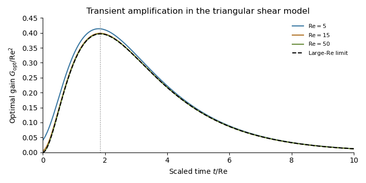
Optimal transient energy gain scaled by Reynolds number squared, approaching its large-Reynolds-number limit
. Details. 
Both eigenvalues of the linear generator, and , are negative. Nevertheless the non-normal matrix transfers the slowly decaying second component into the first before viscous decay wins. Modal decay coexists with energy amplification of order over a time of order .
This illustrates transient growth from non-normal modes: large Reynolds number permits much greater disturbance amplification even though the linear stability analysis finds no unstable eigenvalue. The energy-neutral rotational nonlinearity can redirect the amplified state and affect its subsequent evolution. The linear gain alone establishes neither sustained nonlinear instability nor a nonlinear transition threshold.
Articles by others on the same topic
There are currently no matching articles.