Introduce the thermal expansion coefficient , so the linear equation of state is . With gravity , the resting conductive state of Rayleigh-Bénard convection satisfies the steady heat equation and hydrostatic pressure balance. Consequentlyand, up to an arbitrary constant,Indeed , where .
The Boussinesq approximation retains temperature-dependent mass density in buoyancy while replacing it by in inertial coefficients; it requires . Subtracting the conductive state of Rayleigh-Bénard convection and dropping products of perturbations gives the dimensional Linearized Boussinesq equationsThe minus sign in the temperature equation comes from .
Use the thermal-diffusion scaling of a convection layerThe Rayleigh number and Prandtl number areThus the nondimensional perturbation equations areHere is kinematic viscosity, is thermal diffusivity, and positive denotes destabilizing heating from below for .
A direct elimination of pressure gives the same result as taking a double curl of the momentum equation. Incompressibility gives . Apply to the vertical momentum equation and subtract this pressure derivative to obtainHere is the horizontal Laplacian. At , impermeability gives and fixed temperature gives . The stress-free boundary condition gives , since horizontal derivatives of the boundary value vanish. Differentiating incompressibility once in therefore givesFor a horizontal Fourier mode , with real . More generally the nonnegative spectrum of follows by integration by parts for periodic or square-integrable horizontal disturbances. Substituting the separated normal mode gives, with ,The boundary conditions admit a complete Fourier sine series in . For a nonzero horizontal wavenumber, take , , and set . The two amplitude equations areThus the stress-free convection growth-rate polynomial isIts discriminant is , so both growth rates are real for . For , its two coefficients after the leading term are positive: their sum gives , and their product is . Real roots are both negative; nonreal roots have real part . Hence stable heating from above damps every mode. Horizontally uniform thermal modes and uncoupled horizontal viscous modes are also purely damped; impermeability and incompressibility exclude a horizontally uniform nonzero .
Because the unstable-side roots are real, the onset is stationary, an exchange of stabilities in stress-free convection. Setting gives the free-slip convection neutral curveWith , its derivative has the sign of . Its minimum is at , with value . Minimizing also over gives the critical values
Use the Boussinesq approximation with a constant inertial reference mass density , keeping the background mass density gradient in buoyancy. Write and . For , the linearized normal mode equations areThe reference mass density is chosen close to the background values, whose relative variation must be small. Hydrostatic background pressure satisfies .
From incompressibility, . The horizontal momentum equation and the density equation then giveSubstitute these into the vertical momentum equation and multiply by :For , rearrangement gives the Taylor–Goldstein equationThe buoyancy frequency is real for stable stratification, where . Points where are critical levels of an internal gravity wave; the derivation there is understood through a limiting or piecewise formulation. The printed density gradient is , not the pressure gradient accidentally substituted in the local TeX.
Let be the displacement of a material interface and use . On each side, the kinematic boundary condition isThere is one displaced material interface, so its displacement is continuous. Thus the first jump condition isIn particular, vertical velocity need not be continuous when the background velocity jumps.
With no surface tension, pressure continuity applies on the displaced interface, rather than at its undisplaced height. Linearizing gives . Since , this becomes . The horizontal momentum calculation in part (a) givesSubstitute this and to obtain the second jump condition:These jump conditions for stratified inviscid shear flow use one-sided values of and apply to jumps of mass density, vorticity, or velocity. If is continuous, the first condition reduces to continuity of ; a jump of vorticity generally still prevents continuity of . This derivation avoids multiplying singular distributional derivatives of a discontinuous velocity in the Taylor–Goldstein equation.
Take , without loss for this symmetric real base state, and write , , and . The given quartic becomes a real quadratic . Its constant term factors asTherefore exactly whenA negative product means the two quadratic roots are real and of opposite sign: the discriminant is . The negative root gives a pair . One sign has positive temporal growth rate and is unstable. Using the definitions of the hyperbolic functions gives the required unstable band:This proves the unstable band of a three-layer stratified shear flow directly, without needing to solve all four quartic roots.
For the wave interpretation, consider either interface in isolation with decaying normal modes . Put , , and , the intrinsic phase velocity. At either interface , while at the upper interface and at the lower one. The jump conditions for stratified inviscid shear flow give the gravity-vorticity interface wave relationFor stable density jumps, , both intrinsic branches are real. In units , the isolated wave speeds areThe upper wave travelling against its positive background current has . The lower wave travelling against its negative background current has the opposite speed, . Their counterpropagating wave resonance in a three-layer shear flow occurs at , which givesAt large wavenumber, coupling across the separation is exponentially weak, of order . The unstable band becomeswith full width . It is a counterpropagating wave instability: the two waves propagate oppositely relative to their local currents but have almost equal laboratory phase velocities, allowing weak coupling to lock their phases and extract mean-flow energy. The unstable band of a three-layer stratified shear flow thus becomes narrowly concentrated around this resonance. For fixed , arbitrarily large lies outside that band; large- resonance requires to grow with .
Under the convention , a mode's amplitude grows as . The linear stability analysis of real-wavenumber disturbances is therefore summarized byAt there is marginal or neutral hydrodynamic stability: no normal mode grows exponentially, but some may fail to decay. If “linearly stable” includes neutral modes, its condition is . These modal statements do not rule out transient growth from non-normal modes or algebraic growth.
The fixed observer is the ray . The physically selected zero-group velocity saddle defines the absolute wavenumber and absolute frequency :For a smooth frequency branch with , the saddle condition is equivalently . The absolute growth rate isHere and can be complex. A physical saddle point is selected by the localized impulse response and deformation of its Fourier transform contour; an arbitrary algebraic stationary point need not determine absolute hydrodynamic instability.
For a temporally unstable base flow, the relevant saddle growth rate along a ray distinguishes two cases in the chosen observation frame:A convective hydrodynamic instability amplifies a travelling wave packet but lets a localized disturbance decay at any fixed point. An absolute hydrodynamic instability grows at a fixed point. The separating case is marginal in exponential rate and can have an algebraic prefactor. In a frame moving with , replace by : this distinction depends on the observation frame.
In the linear complex Ginzburg-Landau equation, take real. gives advection, carrying the envelope downstream at speed . gives wave dispersion: the imaginary part of the second-derivative coefficient changes wave phase without directly dissipating a real-wavenumber Fourier mode. gives local linear production or damping: a spatially uniform perturbation grows for and decays for .
The real part of the diffusion coefficient is the scaled value one. It smooths the envelope and damps a real-wavenumber Fourier mode at rate . Thus the linear complex Ginzburg-Landau equation models competing advection, smoothing through a diffusion equation, wave dispersion and local growth, rather than nonlinear saturation.
For a normal mode, , , and . Substitution into the linear complex Ginzburg-Landau equation givesTherefore the dispersion relation isFor real , its temporal growth rate is , with unique maximum at . Its real angular frequency is , displaying the separate advection and wave dispersion terms.
The dispersion relation gives the zero-group velocity saddleThus the absolute growth rate is . More generally the saddle growth rate along a ray isso a frame travelling at sees the maximal rate .
For , the three open regions areThe line is the temporal marginal boundary; the parabola is the convective-to-absolute boundary. The Green function of the linear complex Ginzburg-Landau equation has the prefactor , so zero exponential rate on the latter boundary still allows algebraic decay of the impulse response. This is the stability diagram of the linear complex Ginzburg-Landau equation.
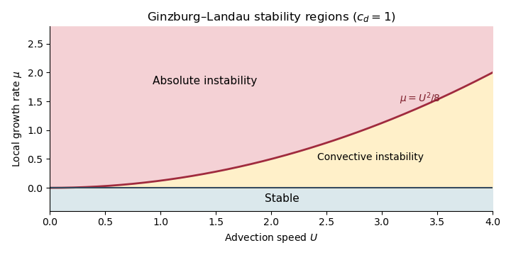
Temporal, convective and absolute stability regions for the linear complex Ginzburg-Landau equation with c_d=1
. Details. 
Impermeability requires . Let with real , and set . If is nonreal, or real outside the channel, the Rayleigh equation for inviscid shear flow gives everywhere. The two wall conditions then force . In fact there is no nonzero globally smooth eigenfunction for any : the complete family is the inviscid Couette continuous spectrum.
For each , permit a localized vorticity sheet. Let be the Dirichlet Green function satisfying . An explicit generalized eigenfunction iswhere and . It vanishes at both walls, is continuous at , and has derivative jump . Consequentlyusing the Dirac delta multiplication identity. These are vorticity-sheet eigenfunctions of inviscid Couette flow, understood as generalized eigenfunctions, not as a discrete smooth Sturm-Liouville eigenfunction expansion.
To see completeness, define the vorticity variable . Its evolution is , so for any admissible initial vorticity ,The homogeneous Dirichlet problem for has only the zero solution, so this inversion reconstructs every initial vertical-velocity field in its usual function space. The generalized frequencies fill the interval with endpoints ; the endpoint values are understood as the closure of the continuous spectrum.
Every generalized frequency in the inviscid Couette continuous spectrum is real: for real . Thus every time factor has unit modulus and there is no exponentially growing normal mode:The vorticity equation also gives , preserving its norm. For fixed nonzero , the bounded Dirichlet Green function inversion therefore gives a uniform bound on the reconstructed velocity in terms of the initial vorticity norm. Superpositions can still rearrange their velocity energy and display transient growth from non-normal modes; neutral hydrodynamic stability does not require every velocity component to decrease monotonically. Treating only smooth discrete modes would miss this continuous neutral family.
Use the kinetic-energy inner product , with perturbation energy . On divergence-free fields the primal generator, before the pressure projection, isThe base state is also divergence-free. The periodic boundary terms in cancel, and decay at removes the remaining boundary terms. Integration by parts changes to ; the Laplacian is self-adjoint under these conditions. Writing , the shear term has adjoint operator . A pressure gradient pairs to zero with a divergence-free field. Hencewhere the last term enforces the divergence-free projection.
To conserve over the finite interval, the physical-time adjoint obeys . Put and ; then . This reverses the interval from towards , or towards .
For , the vorticity cross-product identity and the curl of a cross producthold when both fields are divergence-free. Their difference equals the transport and shear terms in the adjoint operator. Therefore the adjoint linearized Navier-Stokes evolution isThe Leray-Helmholtz projection determines the adjoint pressure. The time-dependent base state is evaluated at ; no extra time derivative of that base state appears in the spatial adjoint operator.
The matrix is a skew-symmetric matrix, so for real . Therefore the energy-neutral rotational nonlinearity contributes nothing directly to the energy balance:The nonlinear term rotates the state without changing its Euclidean norm. It can still change the orientation, and thereby affect later energy growth through the linear term. Thus energy cancellation does not mean the nonlinear and linear trajectories have identical energy histories.
For , the energy balance isThe concave quadratic changes sign at the roots of . For , the neutral orientations and the growth interval areOutside this orientation interval for transient energy growth, the energy decays; at either endpoint it is instantaneously stationary. The direction also has .
In the linear problem, the orientation evolves according to . Since both , a trajectory traversing the positive growth sector has decreasing orientation: growth begins at and ends at , as in the question.
For the full nonlinear model, however,The added rotation can reverse the direction of crossing. Thus the two roots always delimit energy growth, but the printed “begins” and “ends” labels are conditional on a decreasing-orientation passage, and are not universal for arbitrary nonlinear initial conditions.
In the linear problem, , so . Solve with an integrating factor to obtain the complete solution:Equivalently the matrix exponential isBoth eigenvalues of are negative, so each solution eventually decays, despite the possible transient growth generated by .
For the linear evolution from part (iii), maximize the energy ratio at each time. The optimal energy amplification of a linear system isThus the optimizing initial state is a right singular vector, not generally an eigenvector of .
There is a convenient exact way to find the maximizing time. Let be a unit optimizing initial vector and . The singular value decomposition gives . For , the top singular value is simple. At an interior time maximum,Since , this also equals . Thus both initial and final orientations are neutral energy-growth directions. The positive entries of let the top right singular vector be chosen with positive components. Its orientation decreases through the growth sector, so it must start at and end at .
Put and . The solution givesSetting this equal to yieldsTherefore the exact optimal time for isHere and below is the natural logarithm. This is the unique positive stationary time: decreases monotonically from one to zero, and the neutral-direction condition determines one . Also , , and admits initial energy growth, so this stationary point is the global maximum. For , the instantaneous energy-growth criterion for a linear system gives no amplification, and the maximum is one at time zero.
At the optimum, and the initial direction is . Since the final direction has ratio ,Using , , and simplifies this to the exact maximum gain:As , , so and . Consequently the requested large-Reynolds-number transient growth scaling isThese are the optimal time and gain of a Reynolds-scaled triangular model. The leading gain can also be read from the off-diagonal matrix exponential entry: with , is maximized at and has leading maximum .
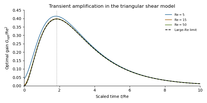
Optimal transient energy gain scaled by Reynolds number squared, approaching its large-Reynolds-number limit
. Details. 
Both eigenvalues of the linear generator, and , are negative. Nevertheless the non-normal matrix transfers the slowly decaying second component into the first before viscous decay wins. Modal decay coexists with energy amplification of order over a time of order .
This illustrates transient growth from non-normal modes: large Reynolds number permits much greater disturbance amplification even though the linear stability analysis finds no unstable eigenvalue. The energy-neutral rotational nonlinearity can redirect the amplified state and affect its subsequent evolution. The linear gain alone establishes neither sustained nonlinear instability nor a nonlinear transition threshold.
Articles by others on the same topic
There are currently no matching articles.