Write . In the local-type primordial non-Gaussianity expansion, the term linear in the short field is . The long-field square contributes to the long background, the mean subtraction is spatially homogeneous, and the short-field square is excluded at the order requested. HenceThis is the long-short coupling measured by a squeezed bispectrum configuration.
Because the long potential is constant over the short-scale region, multiplication by commutes with the linear cosmological Poisson equation and any fixed linear smoothing filter. Thus the short density contrast satisfies . Taking the conditional expected value over the short Gaussian random field givesThe short-scale variance modulation by local non-Gaussianity is conditional on the long mode; averaging over that mode as well would erase the term linear in its zero mean.
Evaluate all derivatives at zero long perturbation, where , and write for the unperturbed abundance. The peak-background split changes the halo peak height toThe chain rule in the specified bias expansion therefore givesNo explicit abundance law is specified, so these derivatives are the general answer. For example, if has the Press-Schechter halo mass function dependence , then and .
For the linear long mode, the cosmological Poisson equation gives . Consequently the deterministic galaxy bias and power spectrum areHere is the linear cosmological density power spectrum; stochastic tracer noise has been omitted. This scale-dependent halo bias from local non-Gaussianity is proportional to in the specified convention.
For , plot the ratio to separate the effect from the shape of . Positive increases the ratio as decreases. Negative first suppresses it, gives a zero when , and then makes it rise again after the effective galaxy bias changes sign. The auto-power spectrum never becomes negative. A truncation is valid only when and must not be extrapolated through the zero. Within the deterministic expression, both signs give at sufficiently small . For a nearly scale-invariant primordial spectrum, in the large-scale transfer limit, so this formal asymptote is .
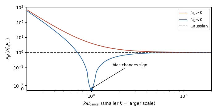
Scale-dependent galaxy bias
. Schematic deterministic power ratio for equal positive and negative coupling magnitudes, with . The negative-coupling cancellation scale defines ; the vertical axis is logarithmic away from a small linear region around zero. Details.
There is a convention issue in calling the specified abundance response an observed galaxy overdensity. The threshold response is naturally a linear Lagrangian halo bias. If instead denotes the physical linear Eulerian halo bias, the Lagrangian-to-Eulerian linear bias relation adds one to the density coefficient: , and . The boxed formulas follow the abundance expansion explicitly supplied in the paper. The Newtonian treatment also cannot be extrapolated beyond its physical large-scale domain without relativistic projection effects.
Use . For nonzero external momenta, the quadratic term in local-type primordial non-Gaussianity isInsert it in one of the three external fields. Wick theorem supplies two connected Wick contractions at each insertion, whereas the mean subtraction removes the disconnected zero-mode contribution. Thus the leading primordial bispectrum isLinear propagation by the cosmological Poisson equation gives and multiplies the primordial bispectrum by . Defining the matter three-point function by its momentum-conserving Dirac delta function times , the primordial contribution to the matter bispectrum isThe nonlinear gravitational contribution from standard perturbation theory in cosmology is excluded here.
In a squeezed bispectrum configuration, , soFor a nearly scale-invariant potential, , so the second term is subleading andRelative to the product of matter power spectra, the squeezed response is enhanced by . Its sign is the sign of . This is the three-point counterpart of the conditional short-scale variance modulation by local non-Gaussianity.
For an attractor with one adiabatic clock and a regular Bunch-Davies vacuum, a long comoving curvature perturbation acts at leading order as a spatial dilation. The single-field inflation squeezed-limit consistency relation therefore fixesFor the local convention , comparison with its squeezed primordial bispectrum givesThe matter-era negative gravitational potential is , so this is also the conventional of part (i). In single-field slow-roll inflation, the spectral tilt is small and the effective local coupling is of slow-roll size, typically of order for a tilt of a few percent. This is a statement about the normalized coupling: the squeezed primordial bispectrum still contains the large long-mode power spectrum.
Formally putting this small coupling into the local template of part (ii) predicts only a tiny correction on accessible scales, rather than an order-unity local signal. For a physical halo abundance there is a stronger qualification. The consistency-relation modulation at fixed coordinate wavelength is a dilation; the coordinate size of a fixed physical halo must be dilated too. Those responses cancel. This is the absence of primordial scale-dependent halo bias in single-clock inflation: the leading consistency-relation term produces no physical halo bias. The first physical long-mode response contains two spatial derivatives, so dividing it by does not produce the local-template enhancement. Thus the leading primordial large-scale galaxy power spectrum remains the Gaussian-bias result, apart from ordinary transfer, bias, and projection effects.
The cancellation can be seen with a top-hat filter. At fixed local time, a constant long curvature rescales physical lengths by , so the coordinate radius of a fixed physical halo is , and the coordinate short density contrast is . Changing variables givesThus the smoothed field and its variance at fixed physical mass are unchanged by the constant long mode.
The assumptions matter: a non-attractor such as ultra-slow-roll inflation, additional fluctuating fields, or an excited initial state need not obey this squeezed-limit conclusion. A sizable physical local modulation would test the stated single-clock attractor assumptions, rather than every possible one-field model.
The background Einstein-de Sitter universe satisfies and . Introduce and for the spatial convolutions in the Fourier transform representation with kernels and , respectively, so and . Differentiation givesAt first order the cosmological continuity equation yields , while the cosmological Euler equation gives . The growing-mode normalization therefore gives .
At second order, take the unsymmetrized order of the inputs printed in the paper. Matching the alpha mode-coupling kernel and beta mode-coupling kernel terms givesHenceWith the paper's unsymmetrized convention , one possible unsymmetrized representation isOnly the symmetric part enters a convolution of two identical linear fields. Symmetrizing givesThis is the one-dimensional cosmological density kernel. The physical symmetric one-dimensional Euler kernel is also : symmetrizing the printed reproduces it, so its apparently different unsymmetrized form is not a contradiction. Unsymmetrized kernels themselves are not unique, since antisymmetric parts integrate to zero. Zero input momenta require the usual separate treatment of the homogeneous background.
Use signed one-dimensional external momenta , with nonzero . Let be the linear cosmological density power spectrum at the time of evaluation, normalized by . Using absorbs the factor multiplying a product of three initial power spectra. All kernels below are symmetrized one-dimensional cosmological density kernels.
The connected B222 contribution to the one-loop matter bispectrum has a triangular Feynman diagram: each second-order external field has two Gaussian inputs, joined pairwise to the other two vertices. The connected B411 contribution to the one-loop matter bispectrum has a fourth-order vertex joined to both linear external fields, with its remaining two inputs contracted into a loop at that vertex. External stubs indicate the measured momenta; blue internal lines represent linear power spectra.


There are connected Wick contractions in the triangle, givingFor a fixed fourth-order external field, attaching the two labelled linear fields gives choices; the remaining pair contracts uniquely. ThereforeThese are contributions to the reduced connected one-loop matter bispectrum, with its external momentum-conserving Dirac delta function removed. Disconnected contractions have a zero external momentum and are excluded.
For the ultraviolet behaviour, the three denominators multiply to a negative square. In factThus for and a smoothly varying high-momentum spectrum,Each second-order vertex exhibits the ultraviolet softness of the second-order density kernel, so this term contains six powers of external momentum.
The fourth-order kernel is even simpler:With a hard-loop cutoff , defineThe B411 contribution to the one-loop matter bispectrum from this range is exactlyFor fixed momentum ratios, it has two external derivative powers multiplying two long-mode power spectra, rather than the six-derivative stochastic structure of . It is the leading deterministic UV-sensitive contribution for external modes below the nonlinear wavenumber. This is a comparison of derivative orders and generic cutoff sensitivity; an arbitrary specially chosen spectrum or vanishing shape can change their numerical ranking. A convergent integral can still depend on nonperturbative short scales. For a high- power law , the integral diverges for , whereas the integral diverges only for , with logarithmic divergences at the thresholds.
At the field level, there are six ways to contract a hard pair within . Comparing with givesThe appropriate second-order density Laplacian counterterm is thereforeIndeed its contribution with two linear fields is , which cancels the displayed hard-loop term. The counterterm sign follows from . Its finite coefficient must be matched to short-scale dynamics, as in the effective field theory of large-scale structure. A term proportional to similarly renormalizes a linear response, but a purely linear insertion cannot by itself cancel this shape, since an odd Gaussian three-point function vanishes.
For one Fourier mode, put . The collisionless equation becomesUse the unweighted Legendre polynomial expansion specified in the paper: . The Legendre polynomial recurrence relation saysThe coefficient of in receives contributions from and . Dividing by gives respectively and . The metric sources are and , the latter becoming after division by . Hence the neutrino Boltzmann hierarchy isThe lower-neighbour term is absent for . The low moments areThese coefficients depend on the expansion convention. In the convention with a factor, the temperature multipoles are ; using those multipoles without converting them would give incorrect factors in the scalar neutrino anisotropic stress.
Let . Rotations around and the vanishing trace imply that the angular integral in the scalar neutrino anisotropic stress has the form . Contract with and use . By the Orthogonality of Legendre polynomials,Only the quadrupole in the neutrino Boltzmann hierarchy contributes. Its phase factor is , so the supplied stress definition becomesComparing with the chosen normalization givesThe sign and factor here follow jointly from the stress convention and the unweighted Legendre polynomial coefficients; they should not be transferred unchanged to a differently normalized hierarchy.
Write . For regular adiabatic initial conditions during radiation domination, use , , and constant potentials. The dipole equation in the neutrino Boltzmann hierarchy givesRegularity removes a constant dipole, and integration yieldsThen the quadrupole equation givesIts regular initial value is zero, soFor the usual regular growing solution, the monopole has no linear correction and parity improves the dipole and quadrupole errors to and , respectively. The weaker bounds above already follow from the assumptions explicitly given. Although the quadrupole is small on superhorizon scales, the trace-free Einstein field equations divide its stress by , allowing a finite leading potential difference.
For one Fourier mode, the trace-free differential operator in the Einstein field equations is , with . Part (ii) gives . The two minus signs in the field equation therefore implyInsert . During radiation domination, , , and the Friedmann equation gives . ThusThese are the radiation-era adiabatic potentials with free-streaming neutrinos; photons are taken to have negligible scalar anisotropic stress.
To normalize the potentials, use . The denominator in the comoving curvature perturbation becomesWith , the conserved curvature therefore obeys . Combining it with the potential ratio givesAs a sign and normalization check, gives . Increasing the free-streaming radiation fraction increases while preserving the supplied curvature convention. The TeX's malformed definition of is restored by the PDF: .
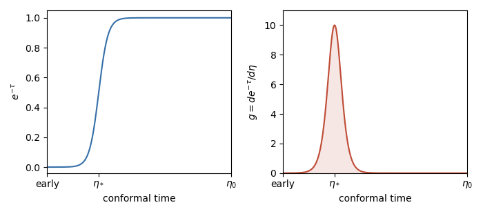
Put , the Thomson scattering rate per unit conformal time. The cosmological optical depth is the integrated scattering rate from emission time to observation, so a Poisson scattering process has survival probabilitySince , the cosmological visibility function isA photon scatters in an interval with rate factor and then reaches us without another scattering with probability , so is its probability of last scattering in that interval. For an optically thick initial epoch,If the initial optical depth is finite, the missing weight represents photons that have already stopped scattering before .
Before cosmological recombination, the optical depth to the present is enormous: , and is also small because almost every scattering is followed by another. Through photon decoupling, rises rapidly and has its dominant positive peak. After decoupling, without reionization, is close to one and reaches exactly one at , while is small because the remaining electron density and scattering rate are small. Residual ionization can give a weak tail; there is no second reionization peak. The peak marks the Cosmic microwave background last-scattering surface.

Let and let differentiate along the unperturbed photon trajectory. Use to decompose the Thomson scattering gain term:The Orthogonality of Legendre polynomials identifies as a pure photon quadrupole. Dropping is an approximation, justified when tight coupling makes the scattering quadrupole small; the supplied unpolarized equation already neglects polarization corrections. The Cosmic microwave background line-of-sight solution requested here omits that quadrupole source.
Set . Adding to the Photon Boltzmann equation with Thomson scattering yieldsAlong , the integrating factor is because . ConsequentlyAn early optically thick boundary makes vanish for finite initial perturbations, and . ThereforeHere and are partial time derivatives, not total derivatives along the ray. We work at first order in scalar cosmological perturbations, evaluate sources along the background radial null geodesic in FLRW spacetime, and ignore observer peculiar velocity. Perturbed paths and lensing affect this first-order source solution only at higher perturbative order. A moving observer adds its local Doppler dipole.
The original PDF, unlike the transcribed TeX, also asks for the instantaneous-last-scattering limit and its interpretation. For with no later scattering, and a matter-era growing mode with constant and , the Integrated Sachs-Wolfe effect vanishes. HenceThe four terms are the intrinsic emission temperature, the gravitational potential at emission, the observer's potential, and the Doppler CMB anisotropy. The two potentials describe the gravitational redshift; the observer term is independent of direction and is absorbed into the measured temperature monopole. The intrinsic temperature and emission potential form the Sachs-Wolfe combination. On superhorizon scales for adiabatic initial conditions in matter domination, , giving the ordinary Sachs-Wolfe effect . The Doppler sign is positive with the paper's propagation direction ; the viewing direction is .
Write and . Under the stated matter-era growing-mode approximation, , and ignoring velocities removes the Doppler CMB anisotropy. The two peaks of the cosmological visibility function give the Cosmic microwave background line-of-sight solutionApply the same solution with observation time , just before the thin reionization screen. Between recombination and that screen there is no further scattering, so free propagation givesA direction-independent potential commutes with the angular average. Thus the incoming photon monopole plus the potential at the screen isSubstitution givesThis derivation inherits the neglected scattering quadrupole and polarization assumptions of part (ii); the screen is an idealized isotropizing approximation.
For a plane Fourier mode , the angular average is explicit:where is the zeroth Spherical Bessel function. The mode's observed transfer isIf , the rescattered monopole is suppressed by at least , because the incoming directions sample incoherent phases. If , and the two propagation phases agree to leading order. The two weights then sum to one. ConsequentlyThese are the small-scale damping and large-scale coherence limits of reionization damping of cosmic microwave background temperature anisotropy.
Each small-scale primary temperature amplitude is multiplied by , so its Cosmic microwave background power spectrum is multiplied by . Holding transfer parameters fixed,Many measured high- modes determine this combination accurately. Their derivatives and are degenerate: a change leaves the leading temperature spectrum unchanged. The undamped large-scale modes can distinguish the parameters, but there are few of them and cosmic variance gives fractional full-sky uncertainty per multipole. This explains the primordial-amplitude–optical-depth degeneracy. Polarization from reionization, lensing, and more complete late-time effects partly break it. The TeX's final is a transcription mismatch; the PDF uses consistently.
Articles by others on the same topic
There are currently no matching articles.