There are two positive roots for : the derivative of is , so the function decreases to its minimum at and then increases. Negative cannot solve the equation. For the larger root, expansion of the exponential function in givesso series reversion yieldsFor the smaller root, set and take a logarithm. Then , so successive substitution gives andThese are the first two nonzero terms of the two asymptotic expansions. Equivalently, the roots are and , from the real branches of Lambert W.
The three fixed- estimates below cease to be uniform as the minimum of the phase approaches the endpoint. For the cubic endpoint-to-saddle transition, writeThe Taylor series of the hyperbolic sine gives, for bounded and fixed ,The cubic term controls the tail, so localization of the Laplace integral gives the uniform leading formulaHere is the cubic Laplace transition integral, equal to in terms of the Scorer Hi function.
To recover the endpoint regime, let . Scale in ; the cubic term becomes negligible and . Thereforewhich agrees with part (i) in the overlap . At , the Gamma integral gives , recovering part (iii).
For , set . The exponent has its maximum at , with second derivative . Thus Laplace's method givesand the transition formula becomesFor with , part (ii) hasPutting reproduces both the exponential and its prefactor. For relative agreement of these leading exponentials, one may use the overlap , which makes . Thus the same transition integral connects all three regimes.
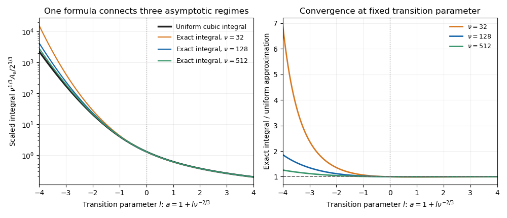
The cubic endpoint-to-saddle transition
. Direct numerical integration of the original phase approaches the same cubic transition function as the large parameter increases. Negative transition parameter places the minimum inside the interval; positive parameter leaves an ordinary endpoint minimum. Details.
Let . For , on the integration interval, so its minimum is the endpoint . The Taylor series isOn the contributing scale , the higher terms are negligible. The endpoint form of Laplace's method, or the Watson lemma, therefore gives
For , the phase has an interior minimum atThe inverse hyperbolic cosine selects the positive stationary point. At this point,Expanding the phase to second order and evaluating the resulting Gaussian integral by Laplace's method yieldsThe exponential grows because the minimum of is negative; the original integral remains convergent because dominates at infinity.
At , the endpoint is degenerate: . The contributing width is therefore , rather than the width in part (i). With , the formula for a degenerate endpoint in Laplace's method givesThe coefficient is a Gamma function value obtained by the Gamma integral.
At fixed , the leading equation is . Its solution compatible with the eventual decaying far field and the boundary value at one is . This decay implies at distances . Balancing radial derivatives against the linear screening term identifiesThe distant region is governed by the modified Helmholtz equation; its decaying homogeneous profile is .
For a matched asymptotic expansion, write the fixed- approximation as , allowing logarithms of in the coefficients. Successive equations areThe boundary condition imposes and . Before matching, their integrated forms can be writtenIn particular a pure power series with parameter-independent coefficients will be insufficient: the logarithmic overlap creates a switchback term.
In the distant region set . The scaled equation is , soDecay and leading matching give . The radial modified Helmholtz equation gives the supplied particular integral in terms of the exponential integral:As , the small-argument expansion of the exponential integral yieldswhere is the Euler--Mascheroni constant. Substitute to compare the two expansions in :The constant at order fixes . Its coefficient then fixes , and the constant at order fixes . HenceThe required inner expansion at fixed isAt fixed positive , the outer expansion isBoth display every term through the requested order, including the switchback term in the fixed- region.
To form an additive composite expansion, subtract the common overlap from the sum of the inner and outer expressions. Their retained common part isThus one composite is . The last term can be screened by multiplying it by without changing either retained expansion. This gives a useful exponentially decaying version:Its boundary value is . If exact satisfaction of the boundary value is desired, use insteadThe small-argument expansion of the exponential integral shows that this normalized composite has the same two retained expansions; it equals one at and tends to zero at infinity.
The linear dispersion relation for a mode is . The proposed modes share phase velocity , so . A quadratic wave interaction generates the second harmonic and the difference harmonic. With only two positive wavenumbers, phase matching for a quadratic wave interaction requires . Equating their phase velocities givesand thereforeThis is a two-to-one resonance of dispersive waves. Its amplitude changes accumulate on . Choose the slow time ; this harmless constant rescaling makes the later amplitude formulas simple. With , the leading real field is .
For the fundamental, the order- cross derivative in is , while the fundamental coefficient in is . For the second harmonic the corresponding terms are and . The solvability condition in the method of multiple scales removes the resonant forcing and givesThe nonresonant third and fourth harmonics enter the correction. They do not change these leading amplitude equations.
Write , and . Taking real and imaginary parts gives the explosive two-to-one amplitude system in polar form:The polar phases are used where their corresponding amplitudes are nonzero. These equations implyFor the second identity, differentiate using : the terms proportional to cancel. Thereforeare first integrals, and in particular
For constant phases with , these real equations reduce to and . The initial data give , so the Riccati equation for is . Integrating and using givesThe tangent and secant function have a pole at , corresponding to . Both modes grow through their locked resonant interaction. This is formal finite-time blowup of the reduced amplitude equations; the weakly nonlinear expansion loses validity as the amplitudes become large, so it cannot establish a singularity of the full partial differential equation.
Interpret the displayed two-harmonic form as a leading term in a weakly nonlinear expansion. Write and . The linear operator multiplies byFor , this is and , respectively. Thus detuning of a wave resonance enters at the same order as the quadratic forcing. The cosine addition formula givesProjection onto the two resonant harmonics by harmonic balance requiresThe nonzero branches are thereforeThe two signs are related by a half-period translation of ; the trivial branch also exists.
The nonresonant first correction supplies the generated mean, third harmonic and fourth harmonic. Their linear multipliers at are , giving the nonresonant partFurther resonant amplitude corrections are determined at higher order. Consequently the nonzero answer describes an asymptotic periodic travelling wave with additional harmonics. Literally retaining only the two displayed harmonics cannot be an exact nonzero solution: their square has a positive constant term, while the linear operator applied to the two cosines has no constant term. The distinction is essential to interpreting this perturbative ansatz.
Articles by others on the same topic
There are currently no matching articles.