A matched asymptotic expansion constructs approximations in regions with different distinguished limits and fixes their free constants by requiring agreement in an overlap region. The inner expansion resolves rapid variation; the outer expansion describes the surrounding region. Matching compares their common limiting behavior, rather than imposing distant boundary conditions directly on a local approximation.[ref]
Asymptotic Analysis and Singular Perturbation Theory by John K. Hunter. §§4.3.3–4.3.4, pp. 57–58: inner expansion and matching
For the singular perturbation problem , , , the leading outer solution is . The inner variable gives and , hence . In the overlap region , the inner variable tends to infinity while the outer coordinate tends to zero. The asymptotic matching condition isso . One concrete path through the overlap region is : then and . Matching selects the free constant that the left boundary condition alone could not determine.
Why choose the right boundary condition for the outer solution? If instead one selects from the left, a proposed right boundary layer with satisfies . Its general solution is . Matching to zero as forces , contradicting . The direction in which the exponential function decays determines which endpoint can carry the boundary layer; endpoint selection is part of the calculation.
For , , , the exact outer solution is and the mismatch is at the right endpoint. In , matching gives and . Differentiation at gives the displayed endpoint slope. The order-one term requires the first inner correction; differentiating only the leading boundary layer loses it.
A growing linear mode can make a formally small derivative nonlinearity order one at large distance. After the crossover scaling, the equation reduces to a logistic differential equation in for . Matching at small gives and the displayed primitive with . It changes from quadratic growth to linear growth without a finite turning singularity.
When the early growing solution is and the nonlinear coefficient depends on , its crossover occurs at the displayed scale. If is order one this is ; if the initial slope suppresses the leading mode and , it is delayed to . The first nonzero perturbative seed must therefore be computed before constructing the global leading approximation; setting the small parameter to zero can erase the mode that ultimately dominates.
For , matching , fixes the first integral to . Hence endpoint values above cannot match this outer branch. The upper family is . An endpoint value strictly between and admits two translations, one initially approaching and one initially moving towards the turning value . Values below give the unique lower family with . Matching to zero instead gives , which forbids a nonconstant real approach to zero. These are leading boundary layer classifications, not exact multiplicity theorems at degenerate endpoint data.
In , balancing all three terms where the outer branches and meet gives the displayed dominant balance and the inner equation . Matching to and writing gives . Its linearized decaying correction is an Airy function; the growing correction is excluded. Matching to zero instead gives , whose nonzero Airy function combinations oscillate. Thus the acceptable matching branches differ qualitatively at the turning endpoint.
An asymptotic matching condition requires the inner expansion and outer expansion, re-expressed in a common overlap region, to agree to the retained order. Both function values and slopes may constrain the free constants. In the square-root reaction problem with nested boundary layers, the shared small plateau sets the first integral of a square-root reaction layer, while its large-field fourth-power tail fixes the neighboring broad layer.
For fixed and endpoint values , , the outer solution is . The left boundary layer has width . At the right, a layer of width carries the order-one rise, and a translated layer of width connects its inner edge to the small plateau. The dominant balance depends on both amplitude and derivative scale; using the same scale at both ends loses a necessary match.
After and or a translated version, the layer equation is . Multiplying by and matching , fixes the energy constant to and gives the displayed factorization. The increasing branch below approaches it at positive infinity; the increasing branch above it leaves it at negative infinity and grows like . This supplies both interfaces of the square-root reaction problem with nested boundary layers.
Multiplication by makes this example exactly integrable once: . Its homogeneous solution is . A solution with that remains uniformly bounded needs , hence . The scales and connect the small outer solution to the order-one endpoint value. Bounded homogeneous contributions remain invisible to algebraic matching at the right boundary.
A decaying algebraic tail in an inner asymptotic expansion can become a fractional-order outer correction after rescaling. For an inner tail proportional to and outer variable , the outer correction is proportional to . If the next outer correction contains , expressing it in the inner variable produces both and . Omitting the latter loses a term larger than a plain correction. Matching must include all these scales and constants, rather than only the leading algebraic powers.
In a singular first-order equation with coefficient , an outer correction proportional to cannot be evaluated at the endpoint. The inner scale changes it to . Matching retains the logarithmic constant, which is larger than a plain order-epsilon correction. For , , the exact solution verifies the displayed endpoint asymptotic and its remainder.
The equation integrates to . Equal endpoint data force and give the unique Gaussian solution above. Its central width is , with amplitude . The exponentially large central mode is missed by an assumed bounded algebraic outer expansion . Changes of order one relative to either endpoint value occur over distance from that endpoint.
For on , removing the drift by givesThe transformed potential changes sign at . WKB approximation is oscillatory inside and exponential outside this turning region; an Airy turning-point connection formula applies over width . At the endpoint the wavelength is , while the physical exponential prefactor changes on the envelope scale . Balancing only diffusion and drift and declaring a single layer misses the zeroth-order term and the turning region. Matching constants may be singular at homogeneous boundary-value resonances.
For with smooth bounded positively away from zero, the first-order equation for the outer expansion is selected by the right boundary condition. The left mismatch is repaired on the scale . If , the leading inner transient is . Its next equation is . Matching its constant and linear large- terms to the outer expansion permits an order- composite approximation. A sign reversal of the drift places the transient at the opposite endpoint.
If a leading outer expansion diverges as and a derivative coefficient contains , balancing that nonlinear correction gives a layer larger than . Write with and subtract the large negative constant from . Matching often introduces a correction and yields an endpoint slope of order . The balance must be derived from the actual equation; logarithmic divergence alone does not fix a universal layer width.
For with left endpoint , diffusion there is of size . The distinguished coordinate is , giving . Matching to one with zero left value gives . The layer width is different from the endpoint's distance from zero.
In , the drift vanishes at the endpoint . Balancing diffusion against drift gives the inner expansion coordinate . The leading layer equation is , with a bounded error function profile. A regular outer first-order calculation alone cannot impose both endpoint values.
If an outer expansion contains and the layer coordinate is , its overlap contains . Matching forces an inner expansion term when that homogeneous profile tends to one in the overlap and vanishes at the boundary. The logarithm multiplies the matching profile, rather than an arbitrary constant.
An overlap region is a parameter-dependent range in which two neighboring asymptotic expansions have simultaneously ordered common limits. Between scales and , it is : the narrow coordinate tends to infinity while the wider coordinate tends to zero. Matching uses these limiting descriptions, not an assertion that either expansion is uniform at all values of the other's scaled variable.
An intermediate asymptotic region has a scale between two other scales and provides their connecting matched asymptotic expansion. It can be needed because a coefficient changes its dominant form before the narrowest region's highest-derivative balance is reached. For example, a coefficient changes near even when the fast inner expansion has width . The intermediate solution must be matched at both ends rather than assigned an independent boundary value.
In , a simple zero , , balances diffusion and advection on width . With , the leading homogeneous inner equation is , whose bounded solutions are constants and the error function. Thus distinct order-one outer solutions can match across an interior transition. Reversing the diffusion sign makes the nonconstant homogeneous solution grow at both ends, changing the matching structure.
For on an interval straddling , the bounded leading interior solution cannot connect unequal constants. A common bulk value is instead selected by an inner solvability condition, and width- endpoint layers enforce the two boundary values. At endpoints with , their leading decaying factors are and . The interior layer still corrects derivative mismatches at smaller amplitude.
A distinguished limit rescales variables so that two or more effects enter the leading asymptotic balance together. It identifies a region whose governing equation differs from the equations in adjacent scales.
An inner expansion resolves a region in which a stretched independent variable makes otherwise small effects enter the leading balance.
The singular perturbation equation balances its derivatives on the width . The inner equation is , so . Its solution with and is the displayed , since . Near zero , so the first derivative is finite while the second is singular. Treat the differential equation on the open interval and impose the endpoint value by continuous extension.
An inner variable is a stretched coordinate such as that remains order one inside a thin region of width . Its scale is chosen by a dominant balance, rather than by the size of a coefficient alone.
For the singular perturbation problem with , , set and . The chain rule givesThus both derivative terms survive in the inner differential equation . The exact domain is , withFor bounded , as : the inner expansion has a nonconstant limiting profile even though the outer solution is constant. The finite- profiles nearly collapse onto after rescaling, with their remaining difference coming from the normalization at the distant right endpoint.
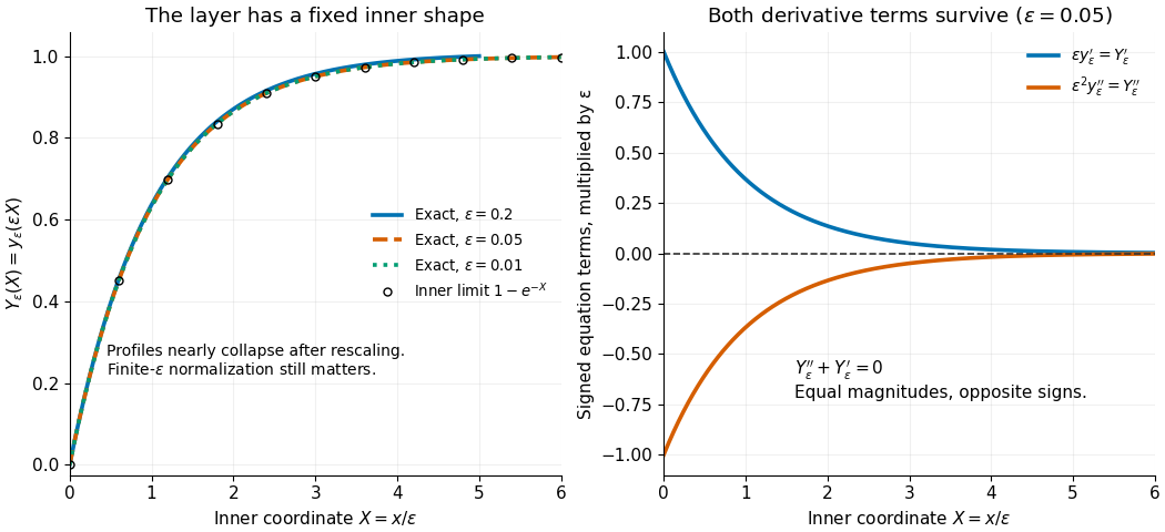
Inner rescaling reveals the common profile and derivative balance
. Left: the exact normalized profiles nearly coincide as functions of the inner variable ; the curve ends at , its actual right boundary. Right: multiplication of the original differential equation by gives the signed terms and , which cancel exactly. Details.
An outer expansion describes the solution away from a thin or distant region resolved by an inner expansion. It is matched to that inner expansion in their common overlap region. Its range of validity must be specified: an approximation at each fixed positive need not have uniform convergence down to an endpoint.
For the singular perturbation problem , , , try the asymptotic expansion at fixed . Substitution gives and for . Expanding the right boundary condition gives and for . Therefore and every higher coefficient vanishes. The missing boundary layer is exponentially small at each fixed positive , invisible to all these powers of .
The exact solution supplies a quantitative limit. For every fixed ,This is uniform convergence on . On the same supremum norm of the error is exactly one. The inner expansion supplies the endpoint information that this outer expansion cannot encode.
An additive composite expansion combines an inner expansion and an outer expansion by subtracting their common behavior in the overlap region:The subtraction removes the part counted twice. Near the boundary layer, the outer expansion cancels the overlap contribution; away from the boundary layer, the inner expansion cancels it. An error estimate is needed to establish accuracy across the whole domain.[ref]
Asymptotic Analysis and Singular Perturbation Theory by John K. Hunter. §4.3.5, p. 58: uniform solution and overlap subtraction
For the singular perturbation problem , , , the outer solution is one, the leading inner expansion is , and their overlap is one. Thus . With , comparison with the exact normalized solution givesThe supremum norm error is therefore exponentially small on the entire interval, even though the outer solution alone has error one. This is an error bound for function values; errors in derivatives have additional powers of .
The composite satisfies the differential equation exactly but has right boundary condition . Dividing it by restores that boundary condition and recovers the exact solution. This example makes both the strength and the limit of matching explicit: it gives a global approximation, while finite- normalization can still carry information beyond every algebraic order.
When inner and outer approximations share a nonzero multiplicative overlap, a multiplicative composite divides their product by that common part. It is especially convenient when different regions contribute separate exponential or boundary-layer factors.
For with , the reduced first-order outer problem takes its boundary condition at the right endpoint. A rapidly decaying exponential in supplies the otherwise unsatisfied left-end condition, so the layer lies at the outflow end for the fast mode associated with this sign convention.
A switchback term such as is forced into a matched expansion when logarithms of a stretched coordinate split into parameter-dependent and local pieces in the overlap region.
If a stretched variable is and an outer expansion contains , its expression in the fixed- region is . The parameter logarithm must therefore be present in the inner expansion, often multiplying a homogeneous solution selected by a boundary condition. An ansatz containing only integer powers with parameter-independent coefficients misses this switchback term. The same reasoning applies to other powers of and other stretched-coordinate scalings.
Articles by others on the same topic
There are currently no matching articles.