The arrival phase has a uniform distribution over a cycle of length . The no-delay phases occupy length , soIndividual phase endpoints have probability zero. The model neglects clearance time and releases waiting vehicles together when the stop interval ends; the degenerate case is interpreted as release at successive cycle boundaries.
For a stop-phase arrival at time , the delay is . An interval of delays of width therefore corresponds to an interval of arrival phases of the same width, because . Its unconditional probability is . Hence the positive-delay part has densityThis ordinary density integrates to , not to one: the remaining probability mass is at . Thus has a uniform distribution with an atom at zero, with mixing weight . Conditional on a positive delay, the density would instead be on .
The graph of the positive-delay probability density function is a horizontal segment at height from to , followed by zero from to . Values at individual endpoints do not affect probabilities. The separate atom at zero is not a finite-height part of this density graph.
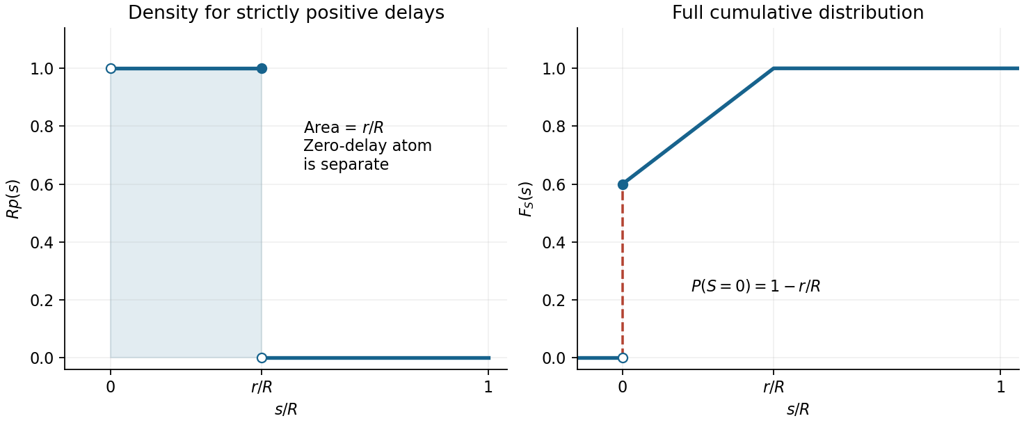

The companion cumulative distribution function in the figure is for , for , and for . Its jump at zero displays the discrete part without confusing density height with probability mass.
The probability of a positive delay is the integral of its density:Adding the separate no-delay event givesThis is the normalization of a probability distribution with both discrete and continuous parts.
The atom at zero contributes zero to the expected value, while all positive delays must retain their unconditional density. ThereforeThis mean is times the mean conditional on encountering a stop; using alone would omit the vehicles passing without delay.
The second moment isSubtracting the squared expected value gives the variance and standard deviation:The variance is nonnegative because . Both and have units of time. At the result reduces to , the standard deviation of a uniform distribution over one full cycle.
Condition throughout on the given arrival time of A, with . A departs at time . B also departs at exactly when it arrives before that release, so , or . Since is uniform on an interval of length ,The original timeline below shows the three disjoint ranges of . The same idealized simultaneous-release convention as in part (a) is used.
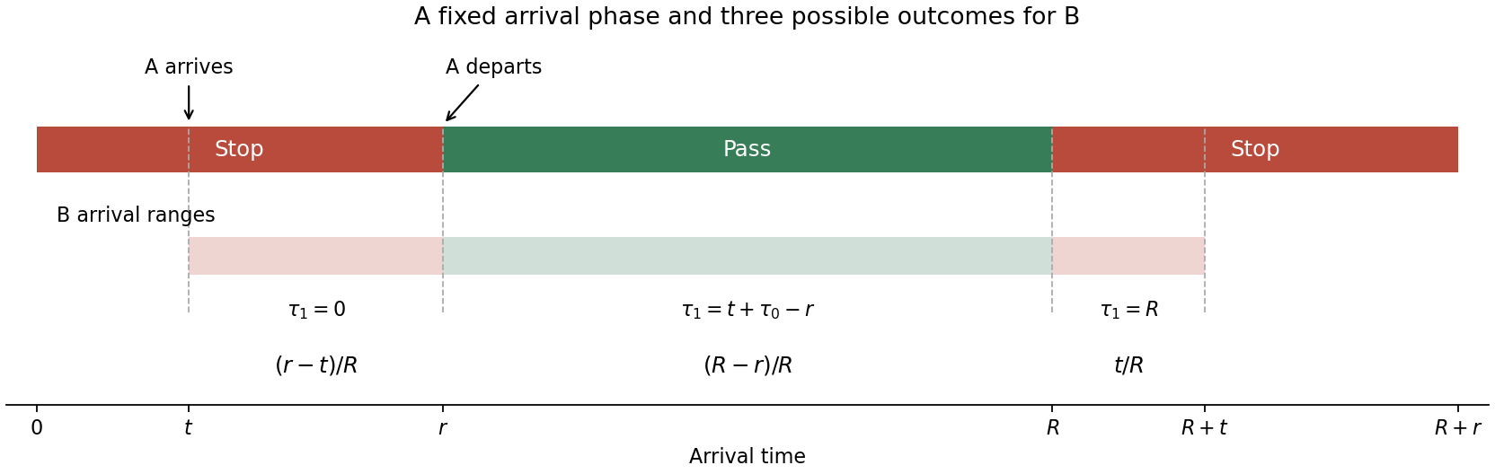
Conditional arrival ranges for the following vehicle at a fixed arrival phase of the leading vehicle
. Details. 
If B arrives during the remaining pass phase, then , or . It passes immediately, soBecause , this is strictly between zero and . The phase interval has length , giving
The remaining arrivals occur in the next stop phase: , or . B waits until , while A departed at , giving . This interval has length , henceEndpoint assignments do not affect probabilities. The three outcomes are exhaustive and satisfyThese are conditional probabilities for the stated fixed ; there is no additional averaging over A's arrival phase in the question.
Articles by others on the same topic
There are currently no matching articles.