Past exam of the mathematics course of the year 1 of the natural sciences course of the University of Cambridge / 2016 / Paper 1

The sum-of-cubes polynomial factorization isMultiplication cancels the two mixed cubic terms and leaves precisely the two cubes.

The polynomial factors asThus the repeated polynomial root is $x=2$, of multiplicity two. Its repetition can also be checked from $p(2)=p^{\prime }(2)=0$ and $p^{\prime \prime }(2)=14\ne 0$.

Factor out $-1/2$ and use the method of completing the square inside the bracket:

Since $x^2-1=(x-1)(x+1)$, write the partial fraction decomposition as $A/(x-1)+B/(x+1)$. Matching the numerator gives $A+B=1$ and $A-B=2$, hence

Use the difference of two squares about $10000$:

For $u>0$, the principal inverse tangent satisfies $\arctan u+\arctan (1/u)=\pi /2$: the two positive acute angles are complementary. Taking $u=\pi /4$ therefore makes the argument of the natural logarithm equal to $(2/\pi )(\pi /2)=1$. The requested value is $\ln 1=0$.

In one period, sine equals $-\sqrt{3}/2$ at $4\pi /3$ and $5\pi /3$, and lies below that value between them. Since sine is a periodic function with period $2\pi$, all solutions are:The endpoints are included because the inequality is non-strict.

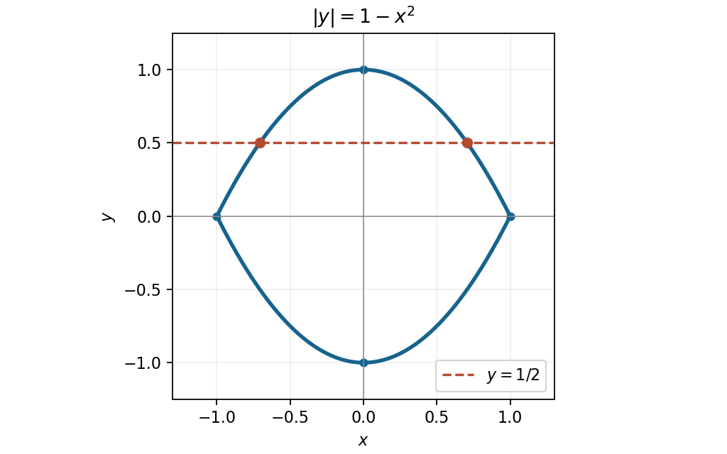
The absolute value is nonnegative, so a real point must satisfy $1-x^2\ge 0$, or $-1\le x\le 1$. On that interval the two branches areThey form a closed lens symmetric about both coordinate axes, meeting at $(\pm 1,0)$ and reaching $(0,\pm 1)$. The parabolas outside the stated interval do not belong to the original locus.

Substituting $y=1/2$ into the absolute value relation gives $1/2=1-x^2$, so $x^2=1/2$. All real intersections are

Separate variables near the nonzero initial condition: $y^{-2}dy=dx$. Integration gives $-1/y=x+C$, and $y(1)=1$ fixes $C=-2$. ThereforeThis is the maximal connected interval containing the initial point. Direct differentiation gives $y^{\prime }=1/(2-x{)}^2=y^2$; the pole at $x=2$ prevents continuation as a finite classical solution of a differential equation through that point.

The derivative of $\cot u$ is $-{\csc }^{2}u$. The chain rule therefore givesThe antiderivative applies on any interval containing no zero of $\sin (3x+1)$.

Additivity of the definite integral combines the adjacent intervals into $[0,n]$. For an integer $n\ge 1$, the power rule givesFor $n=0$, interpret the indexed sum as an empty sum, equal to zero; the displayed expression also gives zero. This convention resolves the otherwise degenerate endpoint of the stated nonnegative-integer range.

The base $2e$ is constant. Write the exponential function as $\exp [\cos x\ln (2e)]$ and apply the chain rule:

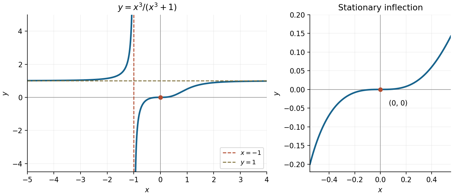
Rewrite the rational function as $y=1-1/(x^3+1)$. It is undefined at $x=-1$, with the vertical asymptote $x=-1$, and tends to the horizontal asymptote $y=1$ as $x\to \pm \infty$. At the pole, $y\to +\infty$ from the left and $y\to -\infty$ from the right.

Its derivative isvanishing only at $x=0$. Since $y(0)=0$ and $y=x^3+O(x^6)$ near zero, this is a stationary inflection point, not an extremum. ThusThe graph increases on each side of the vertical asymptote. The left branch lies above $y=1$, while the right branch lies below it and crosses the origin horizontally.

The first curve is a circle of radius $1$ centred at $(2,1)$. A line through the origin with equation $kx-y=0$ intersects it precisely when the perpendicular distance from that centre is at most the radius. The distance from a point to a line givesHence the full parameter range isThe two endpoint lines are tangent, at $(2,0)$ and $(6/5,8/5)$ respectively; interior values give two real intersections. Both endpoints are therefore included.

The original PDF places a complex modulus around the quotient; those bars are essential. Its denominator excludes $z=-i$. Using $|z^{\ast }-i|=|z+i|$, the case $\lambda =1$ becomes $|z-i|=|z+i|$. In Cartesian coordinates,This locus is the real axis, the perpendicular bisector of the points $i$ and $-i$ in the complex plane. The excluded denominator point does not lie on it.

A quotient with nonzero denominator has zero complex modulus exactly when its numerator is zero. ThusAt that point $z^{\ast }-i=-2i\ne 0$, so the solution is admissible.

For real $\lambda >0$, squaring the two nonnegative moduli gives $|z-i{|}^2={\lambda }^2|z+i{|}^2$. In Cartesian coordinates this isAssume $\lambda \ne 1$ and put $h=(1+{\lambda }^2)/(1-{\lambda }^2)$. Dividing by $1-{\lambda }^2$ yields $x^2+y^2-2hy+1=0$. Since $z{z}^{\ast }=x^2+y^2$ and $b{z}^{\ast }+b^{\ast }z=2\mathrm{Re}(b{z}^{\ast })$, the requested complex equation hasIndeed these choices make the mixed term $-2hy$. Completing the square givesThe Circles of Apollonius therefore haveThe radius is positive for the stated range. No spurious point at $z=-i$ has been introduced: at that point the undivided equation would require $4=0$. Positive $\lambda <1$ gives a circle above the real axis, while $\lambda >1$ gives one below it.

For arbitrary complex $b$ and real $c$, complete the complex modulus square:The locus is a single point exactly when

The same completed square gives $|z+b{|}^2=|b{|}^2-c$. A nondegenerate circle therefore occurs exactly whenFor completeness, $c>|b{|}^2$ gives an empty locus because a squared complex modulus cannot be negative.

No finite choice of $b$ and $c$ gives a line. The coefficient of $z{z}^{\ast }=x^2+y^2$ is fixed at one, so completing the square always gives a circle, a point, or the empty set. A general equation $Az{z}^{\ast }+b{z}^{\ast }+b^{\ast }z+c=0$ could describe a line when $A=0$ and $b\ne 0$, but changing the fixed quadratic coefficient is not permitted here. A limiting sequence of increasingly large circles does not make any one of these finite equations a line.

Write $f(x,y)=F(u,v)$ in the proposed local coordinates. The multivariable chain rule givesConsequentlyAway from the origin the Jacobian determinant is $u_x{v}_y-u_y{v}_x=4(x^2+y^2)>0$, so the inverse function theorem justifies these local coordinates. Therefore $F_v=0$ and the local general solution isSubstitution verifies the result: $f_x=2x{\Phi }^{\prime }$ and $f_y=-2y{\Phi }^{\prime }$, whose weighted sum vanishes.

There is a global qualification. The coordinate map is two-to-one, and a level set of $x^2-y^2$ has separate characteristic curve branches. A single profile on the entire plane does not follow without a branch-identification assumption. For example, take $f=\exp [-1/(x^2-y^2{)}^2]$ on the wedge $x>0$, $x^2>y^2$, and zero elsewhere. This is smooth, satisfies the equation, and has different values at $(1,0)$ and $(-1,0)$ despite equal $u$. The characteristic components of a hyperbolic first-order equation explain this obstruction. At the origin the coordinate map is singular and the original equation reads $0=0$; the boxed answer is the intended local form on a regular branch, or a global form under an additional identification of branches.

The first partial derivatives factor asIf either coordinate vanishes, the other equation forces the other coordinate to vanish as well. If both are nonzero, subtracting the two bracket equations gives $x^2=y^2$, and then $x^2=y^2=1$. Thus the complete list of stationary points is $(0,0)$ and the four points $(\pm 1,\pm 1)$.

The Hessian matrix isAt the origin it is $8I$, which is a positive-definite matrix. At the four other points its eigenvalues are $32$ and $-16$, independently of the signs. The second-derivative test therefore givesThere are no local maxima. The minimum at the origin is not global, since $g(t,t)=8t^2-4t^4\to -\infty$ as $|t|\to \infty$.

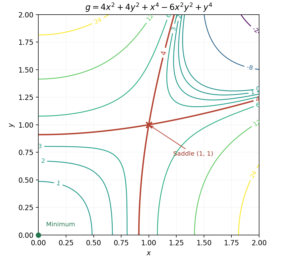
Within the requested first-quadrant square, the stationary points visible in the contour plot are the corner minimum $(0,0)$ and the saddle $(1,1)$. Near the origin, $g\simeq 4(x^2+y^2)$, so the low positive contours look like quarter-circles. Along either coordinate axis, $g=4t^2+t^4$ rises monotonically. Along the diagonal, $g(t,t)=8t^2-4t^4$ rises to $4$ at $t=1$, returns to zero at $t=\sqrt{2}$, then becomes negative.

The saddle contour $g=4$ crosses at $(1,1)$ and separates the central positive contours from the outer diagonal region. Negative contours occur toward $(2,2)$, where $g=-32$, while the axis corners $(2,0)$ and $(0,2)$ have $g=32$. These checks determine both the contour ordering and the change of connectivity at the saddle; the figure shows these level sets.

Write $\mathbf{a}=(a_x,a_y,a_z)$. The cross product gives ${\mathbf{v}}_1=(a_{y}z-a_{z}y,a_{z}x-a_{x}z,a_{x}y-a_{y}x)$, whose three diagonal partial derivatives vanish. For the second vector field, direct differentiation gives ${\partial }_x(2xy)=2y$, ${\partial }_y(x^2+3y^2+z^2)=6y$, and ${\partial }_z(2yz)=2y$. Thus

Put $L=5\pi /2$. The curve tangent is ${\mathbf{r}}^{\prime }=(-b\sin \theta ,b\cos \theta ,c)$. For the first line integral, the scalar triple product identity gives $(\mathbf{a}\times \mathbf{r})\cdot {\mathbf{r}}^{\prime }=\mathbf{a}\cdot (\mathbf{r}\times {\mathbf{r}}^{\prime })$. Its cross product isThe needed definite integrals areand ${\int }_0^L(-\theta \sin \theta -\cos \theta )d\theta =[\theta \cos \theta -2\sin \theta {]}_0^L=-2$. HenceFor the second line integral, substitute the curve into ${\mathbf{v}}_2\cdot {\mathbf{r}}^{\prime }$. The cubic terms combine to $b^3\cos \theta$, leavingThe fundamental theorem of calculus therefore givesBoth calculations retain the full path from $\theta =0$ to $5\pi /2$, rather than inadvertently closing the helix after one turn.

Direct calculation of the curl givesSince $\mathbf{a}\ne 0$, the first vector field cannot be a gradient field: the curl of a gradient is zero. The second is a smooth polynomial field on all of the simply connected space ${\mathbb{R}}^3$, so its vanishing curl makes it a conservative vector field. A potential is also constructed explicitly in the next part. Thus ${\mathbf{v}}_2$ is a conservative vector field and ${\mathbf{v}}_1$ is not. A vanishing divergence alone, as for ${\mathbf{v}}_1$, is a different property and does not establish conservativity.

Integrating ${\varphi }_x=2xy$ gives $\varphi =x^{2}y+h(y,z)$. Matching ${\varphi }_y=x^2+3y^2+z^2$ then gives $h=y^3+y{z}^2+k(z)$. Finally ${\varphi }_z=2yz$ forces $k$ to be constant. A scalar potential isThe initial and final points of the helix are $(b,0,0)$ and $(0,b,cL)$, where $L=5\pi /2$. The fundamental theorem for line integrals givesagreeing with the directly evaluated $I_2$.

By the spectral theorem for real symmetric matrices, choose the normalized eigenvectors to form an orthonormal basis. With $P_n={\mathbf{e}}_n{\mathbf{e}}_n^{\mathsf{T}}$, orthonormality gives $P_n{P}_m={\delta }_{nm}{P}_n$ and ${\sum }_n{P}_n=I$. For every vector $\mathbf{x}$, expand $\mathbf{x}={\sum }_n({\mathbf{e}}_n^{\mathsf{T}}\mathbf{x}){\mathbf{e}}_n$ and apply $A$:Since this equality holds for every $\mathbf{x}$, the spectral decomposition isEach $P_n$ is the rank-one orthogonal projection onto its eigenvector direction. In a degenerate eigenspace, normalized eigenvectors must be chosen mutually orthogonal; normalization alone does not guarantee this resolution of the identity.

The matrix trace is linear, andTaking the trace of the spectral decomposition therefore proves

If every eigenvalue is nonzero, define $B={\sum }_n{\lambda }_n^{-1}{P}_n$, where $P_n={\mathbf{e}}_n{\mathbf{e}}_n^{\mathsf{T}}$. Using the mutually orthogonal projection identity $P_n{P}_m={\delta }_{nm}{P}_n$,The same calculation gives $BA=I$. Thus the matrix inverse is

The inverse fails to exist exactly when at least one eigenvalue is zero. In that case a nonzero eigenvector lies in the kernel of a linear map, so $A$ is not one-to-one. Equivalently, its determinant ${\prod }_n{\lambda }_n$ is zero. Conversely, if every eigenvalue is nonzero, the preceding construction gives an inverse.

The third coordinate is decoupled, giving the unit eigenvector $(0,0,1{)}^{\mathsf{T}}$ with eigenvalue $1$. In the first two coordinates, the symmetric direction $(1,1)$ has eigenvalue $3-1=2$, and the antisymmetric direction $(1,-1)$ has eigenvalue $3+1=4$. Their normalized forms areThey are an orthonormal basis of ${\mathbb{R}}^3$; independent sign reversals are equally valid choices.

Insert the eigenvalues and eigenvectors into the inverse spectral decomposition. The first two projections contributeAdding the third projection givesMultiplication by $A$ gives the identity; in particular the upper block satisfies $\left(\begin{array}{cc}3& -1\\ -1& 3\end{array}\right)\left(\begin{array}{cc}3& 1\\ 1& 3\end{array}\right)=8I$.

Summing the diagonal entries givesThe eigenvalues of the inverse are the reciprocals $1/2,1/4,1$ of those of $A$, whose sum is also $7/4$. This is precisely what the trace identity predicts.

Expand the natural logarithm and reciprocal separately:Multiplication gives the first three nonzero terms of the Maclaurin series:The local expansions converge for $|x|<2$.

The derivative of the inverse tangent is $(1+x^2{)}^{-1}$. Expand it as a geometric series and integrate term by term near zero, using $\arctan 0=0$:

Use $\cosh x=1+x^2/2+x^4/24+x^6/720+O(x^8)$. The Maclaurin series $\ln (1+u)=u-u^2/2+u^3/3+O(u^4)$ givesAll three nonzero terms are needed; stopping at fourth order would supply only two.

Assume the needed derivatives exist continuously and $df/dg\ne 0$ on a neighborhood, so the inverse function theorem provides a local inverse. Put $p=df/dg$, $q=d^{2}f/d{g}^2$, and $r=d^{3}f/d{g}^3$. The chain rule gives $d/df=p^{-1}d/dg$, soDifferentiate once more:Thus the first three derivatives of an inverse function areAll forward derivatives on the right are evaluated at the corresponding value $g(f)$.

Since $a_1=f^{\prime }(0)\ne 0$, substitute the proposed inverse series into the forward one. Comparing coefficients of $f,f^2,f^3$ givesSolving successively yields the cubic series reversion coefficientsThe conditions $f(0)=0$ and $a_1\ne 0$ ensure that both local series are centred at zero and that the inverse has a linear leading term.