An optical soliton maintains a localized profile because nonlinear refraction compensates linear spreading. A temporal optical soliton balances group velocity dispersion against self-phase modulation; a spatial optical soliton balances diffraction against self-focusing. The relevant coordinate and sign of nonlinearity must be specified.
For anomalous group velocity dispersion and positive , a fundamental temporal bright soliton isThe identity verifies both the width relation and propagation phase. Its dispersion length equals its nonlinear length . Bright pulses decay to zero background. dark solitons are intensity depressions on a nonzero background with a phase change across the dip; black dips reach zero intensity, while grey dips do not. For positive the corresponding temporal defocusing regime has normal group velocity dispersion.
A higher-order temporal soliton has soliton order equal to an integer greater than one for the special initial profile in normalized units. It breathes through compression and splitting/recombination, rather than keeping one fixed shape. Separated fundamental solitons can interact and acquire collision shifts. An arbitrary pulse with noninteger is not automatically a pure higher-order soliton; dispersive radiation can carry part of its energy.
In ideal one-dimensional cubic propagation, dispersion and nonlinearity support stable fundamental bright pulses. Loss, higher-order dispersion, delayed nonlinear response and finite bandwidth change real-fibre propagation. A one-dimensional spatial bright solution also does not guarantee stability against two-dimensional collapse. Profile preservation, finite-energy background conditions and robustness should be checked rather than inferred from any solitary-looking peak.
A detector too slow to resolve a femtosecond field can measure its integrated nonlinear response instead. Split the pulse, delay one replica, overlap both in a thin phase-matched crystal, and select the sum-frequency signal. For negligible depletion and sufficiently broad phase matching, the cross-generated field is proportional to ; integrated signal gives the second-harmonic intensity autocorrelationA noncollinear geometry can reject each replica's individual second harmonic. The optical response supplies the fast gate while the detector integrates slowly. Crystal thickness, group-velocity mismatch, spectral acceptance, beam overlap and delay calibration limit resolution.
For a Gaussian pulse specified by its intensity profile, the autocorrelation's full width at half maximum is times the intensity full width at half maximum. For a sech-squared intensity profile the ratio is about . These are model-dependent conversion factors. An intensity autocorrelation is symmetric in delay and loses phase information; different pulses can share it. An interferometric autocorrelation retains rapid carrier fringes but still does not generally reconstruct an arbitrary complex field uniquely.
frequency-resolved optical gating also resolves the gated signal's spectrum, giving a two-dimensional delay-frequency record. For second-harmonic frequency-resolved optical gating,where is measured relative to the signal's carrier. An iterative retrieval seeks an envelope whose predicted record matches the measurement. Alternatively, polarization-gating frequency-resolved optical gating uses the optical Kerr effect to gate the probe by a delayed replica's intensity, with signal envelope proportional to . The original FROG work introduced nonlinear optical gating plus spectral resolution to characterize arbitrary femtosecond pulses.[ref]
Characterization of arbitrary femtosecond pulses using frequency-resolved optical gating by Daniel J. Kane and Rick Trebino. 1993, abstract: nonlinear gating and spectrogram construction
Absolute wave phase and absolute time origin remain undetermined by these intensity records. The SHG record also cannot distinguish from , so its time-direction ambiguity remains. Retrieval agreement, an independently measured spectrum, adequate signal dynamic range and gate-response calibration are practical consistency checks. A pulse train that changes between shots can yield an averaged record that no single pulse faithfully represents. Thus nonlinear gating solves the detector-speed problem but does not remove inverse problem ambiguities or experimental limitations.
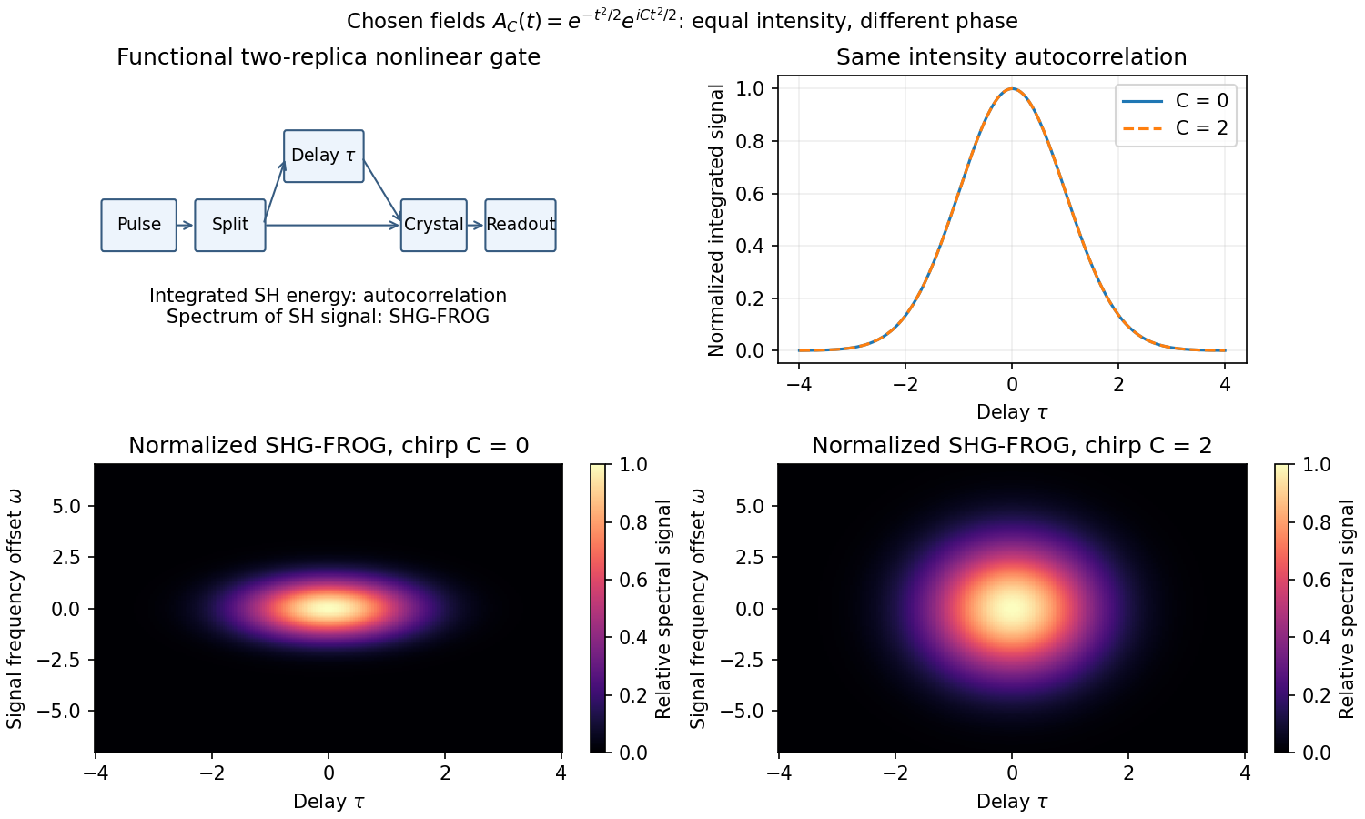
Original nonlinear pulse-gating layout and a calculated Gaussian chirp example distinguishing autocorrelation from spectral gating
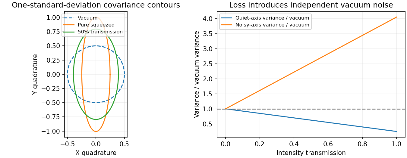
. Details. For and , , so . Vacuum and coherent states have variance in either optical quadrature. quadrature squeezing means that some rotated optical quadrature has variance below this reference, with compensating noise elsewhere. A reduced second moment about zero is not the correct test when the field's mean is displaced.
For and , the quiet principal axis of the optical squeezed vacuum is at angle under the squeeze-operator convention used above, andThe pure Gaussian quantum state saturates the uncertainty product. Displacement moves its centre without changing its covariance ellipse; squeezed thermal states instead have a larger uncertainty product. The optical squeezed vacuum has zero mean field, even photon-number parity and mean occupation ; it need not have sub-Poissonian photon statistics. number squeezing and quadrature squeezing are different conditions.
Degenerate parametric amplification generates single-mode squeezing; a two-mode squeezed vacuum instead has correlated occupations and joint quadrature squeezing. Either individual mode of an ideal two-mode state is thermal after the other is ignored, not individually squeezed. balanced homodyne detection measures the noise versus local oscillator phase. Reference phase drift admixes the anti-squeezed optical quadrature, while electronic noise and detector imbalance need separate checks.
For an optical loss channel with efficiency and vacuum entering the unused port, optical squeezing degradation by loss givesThe linear-loss limit follows directly by writing the output field as with independent vacuum mode . Loss therefore places a floor under measured squeezing. Squeezed input can improve phase-sensitive measurements when aligned with the measured optical quadrature; it does not reduce every noise source or both conjugate uncertainties at once.


Articles by others on the same topic
There are currently no matching articles.