Past exam of the numerical analysis course of the University of Oxford / 2015 / 2 / c

Assume $f\in C^{n+1}[a,b]$ and reorder the interpolation nodes increasingly as $x_0<\cdots <x_n$. The polynomial interpolation error $e=f-p_n$ vanishes at all of them. Rolle's theorem suppliesThese $n$ points are distinct because their containing intervals are disjoint. Thus $q=p_n^{\prime }$ is a polynomial of polynomial degree at most $n-1$ that interpolates the function $f^{\prime }$ at the interpolation nodes ${\eta }_1,\dots ,{\eta }_n$.

Apply the polynomial interpolation error theorem to $f^{\prime }$ with these $n$ interpolation nodes. Since the $n$th derivative of $f^{\prime }$ is $f^{(n+1)}$, for every $x\in [a,b]$ there is a ${\xi }_x\in (a,b)$ withFor $x={\eta }_i$ the equality is zero on both sides; otherwise the same auxiliary-function and repeated-Rolle's theorem proof applies. This also covers $n=1$, where $q$ is a constant polynomial and the proof is the ordinary mean value theorem for $f^{\prime }$.

Writing $M={\max }_{[a,b]}|f^{(n+1)}|$ gives the genuine error boundThe first formula is sharper, but its intermediate interpolation nodes depend on $f$; the last bound eliminates those unknown locations. This is derivative interpolation error from Rolle points.

The remainder in part (b) involves an unspecified $\xi =\xi (x)$. Its existence for every $x$ does not ensure a differentiable selection. Even if such a selection existed and $f$ had an additional derivative, the product rule and chain rule would giveThe first term cannot be discarded or bounded from the given information. Neither $f^{(n+2)}$ nor ${\xi }^{\prime }$ is supplied by the original theorem.

For an explicit demonstration, interpolate the cubic polynomial $f(x)=x^3$ at zero and one. Then $p_1(x)=x$, andDifferentiating correctly givesTreating the remainder coefficient $x+1$ as a constant would omit $x(x-1)$ and give a wrong answer at every interior point. An existential intermediate point cannot be frozen when differentiating. Part (i) instead applies Rolle's theorem directly to the polynomial interpolation error.

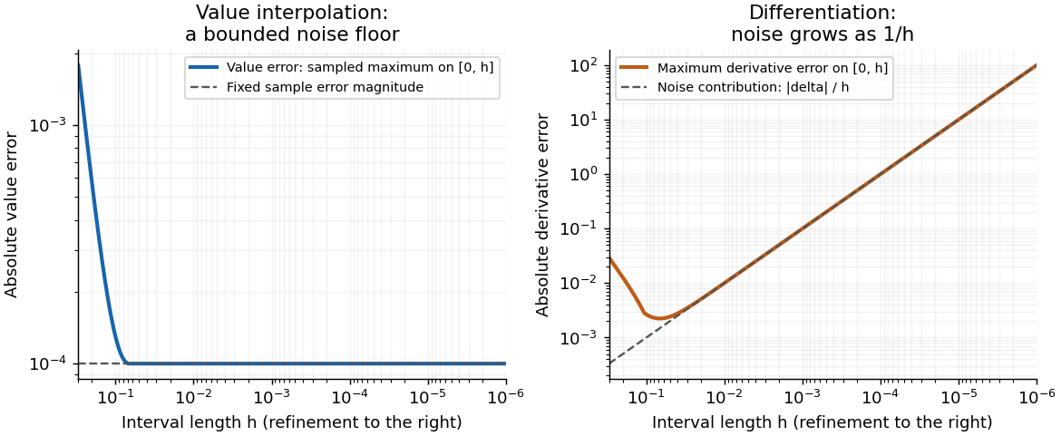
Write ${\tilde{p}}_1$ and $\tilde{q}$ for the quantities computed from the perturbed second sample. The endpoint linear interpolation and its derivative areCompare them on their interpolation interval $0\le x\le h$, with fixed $a>0$. Put $x=th$, $0\le t\le 1$. The Taylor series of the sine gives, uniformly in $t$,Here the second equality compares with $f^{\prime }(0)=a$. More generally, the exact derivative is $f^{\prime }(th)=a\cos (ath)$ andThe input perturbation itself changes the value interpolant by exactly $aϵx/h$, and changes its derivative by exactly $aϵ/h$. ThusFor fixed nonzero $ϵ$, the value approximation has a bounded noise floor: its maximum error approaches $a|ϵ|$, and at $x=h$ that error is exactly $a|ϵ|$. It does not converge uniformly to the exact values as $h\to 0$. However, it does not amplify the absolute sample perturbation on $[0,h]$. The derivative error instead grows without bound like $a|ϵ|/h$.

With exact samples, $ϵ=0$, both approximations do converge on the shrinking interval: the value error is $O(h^3)$ for this particular sine, and the derivative error is $O(h^2)$. With step-dependent noise, value convergence requires $ϵ(h)\to 0$, whereas derivative convergence requires the stronger $ϵ(h)=o(h)$, where $o$ denotes little o notation.

This is noise amplification by differentiation of a linear interpolant. Value interpolation has an absolute perturbation bound independent of $h$ on the sampled interval. Numerical differentiation has a perturbation factor $1/h$, expressing the ill-posedness of numerical differentiation from values with fixed absolute uncertainty. The amplification follows from the mathematical data map even in exact arithmetic; it is distinct from additional roundoff error in a particular implementation. For fixed $x$ outside $[0,h]$, the operation becomes extrapolation, and the value perturbation $aϵx/h$ can also diverge.