At an air–glass interface, resolve the incident unpolarized light into components perpendicular () and parallel () to the plane of incidence. The Fresnel equations give the parallel reflection coefficientAt Brewster's angle, . Together with Snell's law, this gives and . Thus, taking the incident medium to be air,The remaining reflected component has linear polarization perpendicular to the plane of incidence. This assumes a transparent, nonmagnetic glass with negligible absorption.
Let be the intensity from either fibre alone at the observation point, assuming equal output intensities, matching polarizations and negligible drift. The screen samples the relative phase between the two outputs. For an ideal monochromatic laser, first-order optical coherence is complete andThe interference fringes are approximately equally spaced in the small-angle far field, with a slowly varying diffraction envelope. If the output separation is and the screen distance is , the interference fringe spacing is approximately . Equal phases at the two input ends do not ensure a central bright fringe: the extra fibre contributes carrier phase in addition to the free-space optical path difference.
For a finite linewidth, the time-averaged interference signal becomesHere may be defined for the slowly varying field envelope, with the carrier phase already included in . A realistic laser therefore gives reduced interferometric visibility; for , its extrema are and .
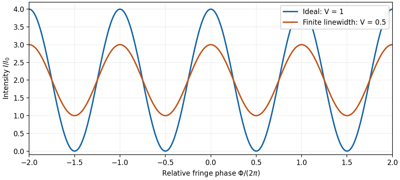
Ideal and finite-linewidth interference for equal output intensities
. Details. 
For a Lorentzian line shape of frequency full width at half maximum , temporal optical coherence givesThe relevant index is the group index. Using the intended nondispersive approximation ,This delayed-fibre linewidth measurement assumes the loss of contrast comes from linewidth. Unequal output intensities, polarization mismatch or mechanical phase fluctuations also lower interferometric visibility. If dispersion matters, the stated phase index alone does not specify the necessary group index.
Use axes adapted to the two orthogonal rotations in the diagram:For a linearly oscillating Hertzian dipole with real unit axis and total time-averaged radiated power , the angular distribution of electric dipole radiation isThe normalization follows from . Equal readings therefore implyHere , since otherwise all components would vanish. Reversing the axis is immaterial, so choose . The complete family isDefine , , and . Then , and the absolute intensity fixesFor the measured distance and intensity, the allowed axes and powers are:
- : , .
- or : , for either axis.
- : , .
The intensity data do not select a unique orientation or total power. This is the dipole-axis ambiguity from three intensity measurements: the readings constrain squared projections and lose their signs. For example, the first branch makes an angle with , but the other branches are equally consistent with the three measurements. A further suitable observation direction or polarization measurement is needed to remove the ambiguity. The calculation uses radiation-zone intensities, as appropriate to the Hertzian dipole model.
Articles by others on the same topic
There are currently no matching articles.