Past exam of the perturbation methods and applied complex variables course of the University of Oxford / 2008 / B / 8

The two holomorphic function functions agree throughout their overlap region strip, so they define a single holomorphic function on the union of their domains, which is the whole complex plane. The resulting entire function is bounded outside a sufficiently large disk by the assumptions at infinity. It is bounded on the disk by continuity and compactness. Liouville theorem therefore makes it constant:Agreement on an open overlap region is what permits analytic continuation; equality of unspecified boundary values alone would need additional hypotheses.

First state the normalization needed for the displayed logarithmic factorization: choose a continuous holomorphic function branch $L=\log F$ in the strip that tends to zero at both horizontal ends and has sufficient decay for its Cauchy integrals. In particular the index of the kernel along a horizontal line must be zero.

Choose $\alpha <c_{+}<c_{-}<\beta$ and let ${\Gamma }_{\pm }=\{\xi +i{c}_{\pm }:\xi \in \mathbb{R}\}$, both oriented from left to right. PutThe first is analytic above the lower line and the second below the upper line. On the region between the lines, closing a rectangle gives $C_{+}L-C_{-}L=L$: the lower horizontal side is traversed forward and the upper side backward. HenceThe equation $F{w}_{+}=w_{-}$ becomes $F_{+}{w}_{+}=F_{-}{w}_{-}$ on the overlap region. With the canonical bounded factors normalized at infinity, these two products glue to a bounded entire function. Part (a) givesThis is Wiener-Hopf factorization with the quotient convention used in this question.

The source hypotheses require a qualification: nonvanishing in the strip and $F\to 1$ do not by themselves force index zero or a logarithm tending to zero at both ends. For exampleis analytic and nonzero for $|\mathrm{Im}z|<1/2$, tends to one at both ends, but winds once around zero along the real line. A logarithm continued along that line changes by $2\pi i$, so it cannot have the stated normalization at both ends. One must first separate the index factor, or allow appropriately subtracted factors and a correspondingly different common-function growth class. The displayed constant conclusion follows under the canonical zero-index assumptions above; it is not an unconditional consequence of the two printed properties of $F$. This is the issue measured by the Index of a Wiener-Hopf kernel.

Use the same normalized factors and contours as in part (b), and put $H=G{F}_{-}$. Multiplying the inhomogeneous equation by $F_{-}$ givesThe additive Cauchy decomposition has $C_{+}H-C_{-}H=H$ on the overlap region. Subtract it from this equation:Under the same convergence and boundedness assumptions, these expressions are analytic on complementary half-planes, agree on their overlap region, and glue to a bounded entire function. ThusIf the decay is too weak for an unsubtracted Cauchy integral, the subtraction and resulting common-function growth condition must be specified. Merely asserting pointwise $G\to 0$ is not a substitute for the needed integral transform convergence.

For $\mathrm{Im}k>0$, put $s=-ik$, so $\mathrm{Re}s>0$. The Laplace transform for the Gamma function, analytically continued from positive real $s$, givesChoose $\arg k\in (0,\pi )$ in the upper half-plane. Since $\arg (-ik)=\arg k-\pi /2$,This integral is absolutely convergent throughout the upper half-plane. On the nonzero real axis it converges conditionally by Dirichlet test for improper integrals, and its value is the upper boundary limit of the same branch. In particular negative real $k$ has argument $\pi$, not $-\pi$ in this formula.

At $k=0$ the integral diverges at infinity; in the lower half-plane its exponential function factor grows and the ordinary improper integral diverges. The origin itself causes no local-integrability problem for $x^{-1/4}$. A useful continuation of the chosen power uses a branch cut descending from $k=0$ with argument in $(-\pi /2,3\pi /2)$.

Use the Fourier transform convention $\overline{U}(k,y)={\int }_{\mathbb{R}}u(x,y)e^{ikx}dx$, initially in a class where the integral transforms and subsequent limits are defined. Transforming Laplace's equation gives ${\overline{U}}_{yy}-k^2\overline{U}=0$ on real $k$. Decay for $y\to \infty$ selectsThe boundary trace is the sum of its negative-half-line unknown and the given positive-half-line datum. The normal derivative is zero on the negative side. ThereforeFor the $e^{ikx}$ convention, negative support gives a integral transform analytic for $\mathrm{Im}k<0$, and positive support gives one analytic for $\mathrm{Im}k>0$, subject to the appropriate endpoint interpretation. The normal trace in this particular problem requires a finite-part interpretation, detailed below.

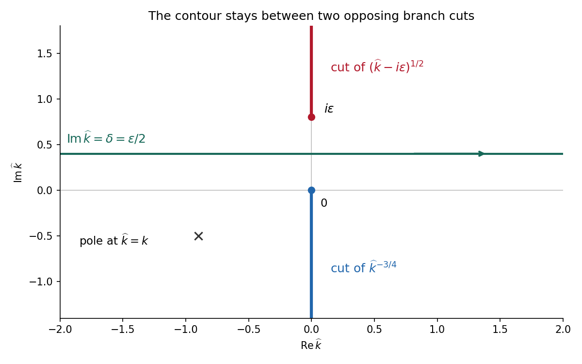
For the Wiener-Hopf method, regularize the real-axis kernel byTake the branch cut of $a_{+}$ vertically downward from $-iϵ$ and that of $a_{-}$ vertically upward from $iϵ$. Their product on the real axis is the positive square root $\sqrt{k^2+{ϵ}^2}$. The branch of $H_{+}$ has its cut downward from zero. Dividing the regularized equation by $a_{+}$ givesThe forcing $P$ is analytic in $0<\mathrm{Im}k<ϵ$, between its two cuts. Decompose $P=P_{+}-P_{-}$ by Cauchy integrals on two horizontal lines within that strip. Separation giveswhen the endpoint growth class makes the common entire remainder bounded. For $\mathrm{Im}k<0$ one can take the minus Cauchy integral on $\mathrm{Im}\hat{k}=\delta$, with $0<\delta <ϵ$, obtainingThe integrand is $O(|\hat{k}{|}^{-5/4})$ at infinity, so the Cauchy integral converges there. In the limit choose $\delta =\delta (ϵ)$, for example $\delta =ϵ/2$; a fixed positive $\delta$ cannot remain between zero and $ϵ$. With $\sqrt{k}$ denoting the limiting lower-analytic branch and with the prescribed limiting interpretation,The numerator square root has a cut going upward from $iϵ$; the power ${\hat{k}}^{-3/4}$ has a cut going downward from zero. The contour passes between them. The pole $\hat{k}=k$ is below this contour when $k$ is in the lower integral transform domain. These branch choices are essential, rather than independent principal powers of the factors.

There is an important mathematical limitation in the source's ordinary integral definition of $\bar{g}$. An explicit harmonic function particular solution in polar coordinates $0<\theta <\pi$ isEach separated polar power is harmonic function; at $\theta =0$ it has the required Dirichlet boundary condition value, and at $\theta =\pi$ its angular derivative vanishes, giving the required zero normal derivative. It also decays at infinity. Its unknown boundary traces areThe last function is not locally integrable at zero. Therefore the printed ordinary integral ${\int }_0^{\infty }g(x)e^{ikx}dx$ diverges, even for $\mathrm{Im}k>0$. The integral transform calculation is valid for this solution only after specifying a Hadamard finite-part integral, or equivalently a distribution boundary trace.

For the canonical homogeneous extension of this power, the two transformed traces areThe first is analytic below and the second above. The second formula follows from $\Gamma (3/4)=(-1/4)\Gamma (-1/4)$ and the finite-part continuation of the Laplace transform. Substituting their real-axis boundary values directly verifies the boxed integral transform relation for both signs of $k$, so the qualification can be checked without relying only on formal factorization.

There is also homogeneous corner freedom:satisfies zero Dirichlet boundary condition data on the positive axis, zero Neumann boundary condition data on the negative axis and decay at infinity. Its negative trace has integral transform $C\Gamma (1/2)(ik{)}^{-1/2}$, corresponding to the term $A/\sqrt{k}$. Higher singular modes $r^{-(n+1/2)}\sin ((n+1/2)\theta )$ would also satisfy the homogeneous boundary conditions for integers $n\ge 1$, but are excluded if the negative trace is required to be locally integrable. Thus the one-constant formula belongs to a specified corner-growth class. The original boundary conditions alone, without that class, do not assert uniqueness. These facts form the finite-part normal trace for mixed quarter-power boundary data.