For each fixed , the next term must be negligible relative to its predecessor:The ratios are understood where their denominators are nonzero near the limiting point, or equivalently through the little o notation definition. For example form an asymptotic sequence.
For every fixed truncation index , the remainder must be smaller than the last retained term:This is an asymptotic expansion relative to the sequence in part (i). The number of retained terms is fixed before taking the limit. The associated series need not converge for any nonzero parameter; its role is to give successively smaller truncation errors. If is an asymptotic sequence, the same condition can be stated as a remainder when the next expansion condition is available, but the displayed little o notation formulation is the defining one.
Take and . Then , so . However,for every , and this ratio does not approach one. Thus asymptotic equivalence need not survive exponentiation. A small relative error between large exponents can leave a nonvanishing additive error. This is the distinction in asymptotic comparison of exponential functions.
The ratio can be evaluated directly:The assumption gives , so continuity of the exponential function givesThe additional premise is not needed for this implication. The useful requirement is additive control of the exponents, as explained by asymptotic comparison of exponential functions.
First take the usual positive-parameter limit . For real , the equation implies , so every root lies near or . Near the positive root,and hence up to an exponentially small correction. Near the negative root, the corresponding limit is minus one, giving to all algebraic orders. Expanding the square roots givesThere is one root in each neighborhood: the derivative has the sign of there for sufficiently small positive . The bound above excludes further real roots.
If the source's unqualified is read as a two-sided limit, use the exact identityThe two-sided versions therefore replace by in both displayed first corrections. The two one-sided algebraic expansions otherwise have the same reasoning.
The function is strictly decreasing from infinity to zero on , so there is a unique positive root, which tends to infinity. Let . Taking logarithms givesFirst . Put with , expand, and cancel :The leading balance gives . Substitution leaves a residual ; the derivative of is of order , so the root error is . ThusThe second term is logarithmic rather than a constant multiple of . This is logarithmic inversion of a Gaussian divided by its argument.
Write and divide the equation by :Balancing the first and third terms gives . With , the terms of order and one giveFor the slow branch , choose and obtain . For the fast branch , choose and obtain . Additive integration constants enter the two independent amplitudes. The two-term WKB approximation is consequentlyImposing the boundary conditions on these two approximating modes yieldsThis uses the first two exponent functions for both branches. The next transport equations, if desired to identify the algebraic error, give for the slow mode and for the fast mode. Thus each displayed mode has relative amplitude correction uniformly on the fixed interval; no turning point occurs because the two leading exponent roots remain distinct.
Dropping the small highest-derivative term gives . The outer solution satisfying the right endpoint condition isIt fails the left endpoint condition, so a boundary layer is needed at . If , diffusion and first derivative balance when , giving .
With , the exact inner expansion after multiplication by isIts leading solution is . The zero boundary value gives , and asymptotic matching condition as , fixes . ThusThe common overlap region value is . Add the outer and inner approximations and subtract that overlap region:The decaying inner exponential function can accommodate the left condition, whereas a right-end inner coordinate would give a mode that grows into the interval. There is no right boundary layer. The composite asymptotic expansion satisfies the left condition exactly and the right one up to the exponentially small term ; the remaining approximation error is algebraic and vanishes as .
Let and introduceDeform the contour upward to the steepest descent contour from zero and the endpoint path from . More precisely the original integral is the first path traversed forward minus the endpoint path traversed forward. Connect the truncated paths where and let . That connector has exponentially small factor , and no pole of is crossed: all its poles are real and outside the original segment.
On the endpoint path , and . Its negative orientation gives the leading endpoint termTaking real parts and inserting givesThe oscillatory first coefficient can vanish at particular values of ; the stated remainder still holds as an additive asymptotic expansion.
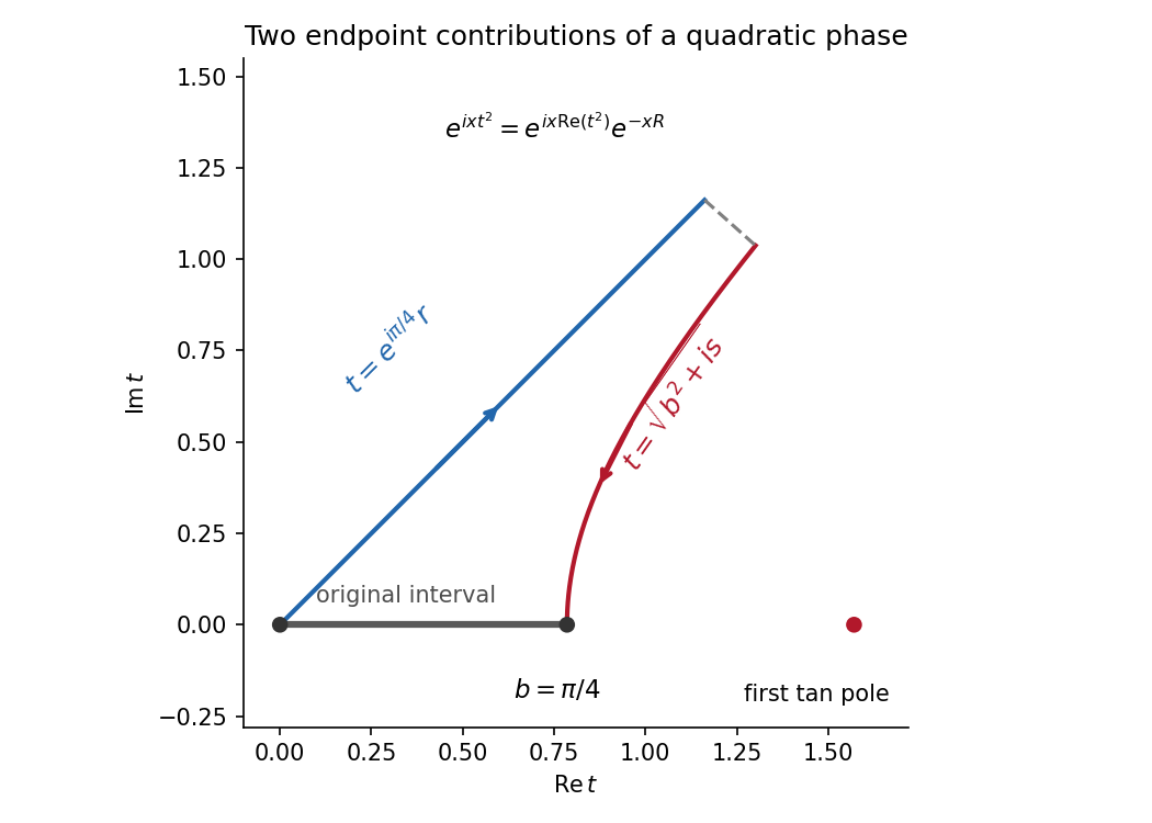
The quadratic phase descends from the stationary endpoint and from the nonstationary upper endpoint
. Details. The only nondegenerate stationary point of a phase of the phase is the endpoint zero. Its usual leading stationary phase method term is proportional to the amplitude there, but . Thus the nominal stationary contribution vanishes.
Expand one order further in the local amplitude: . The rescaling then gives a first nonzero stationary contribution of order , with coefficient in the real integral, as in part (i). Meanwhile the upper endpoint is nonstationary and has nonzero amplitude; its integration by parts contribution is , of order .
Consequently the nonstationary endpoint dominates the first nonzero saddle contribution. A stationary phase method formula retaining only the usual leading saddle term would miss the answer. The full stationary phase method, with the vanishing-amplitude correction and the endpoint term, agrees with method of steepest descent. This is quadratic stationary endpoint with quadratically vanishing amplitude.
Treat as independent variables, with . The chain rule givesTherefore the method of multiple scales isThe unspecified term includes the higher correction in . Only the displayed terms through order are needed to determine the leading slow-amplitude system.
At order one, , soAt order ,The operator sends a constant to itself and sends to minus three times themselves. HenceAn additional homogeneous contribution can be absorbed into the definitions of . There is no resonance forcing at this order; the first amplitude evolution therefore occurs on the chosen slower scale .
The order- equation isUsing and , its resonance coefficients aresecular term are removed by setting these to zero:The eigenvalues of this two-by-two system satisfyThey are real with opposite signs for . Generic initial amplitudes then contain an exponentially growing slow-time component. At either leading endpoint the matrix is nonzero nilpotent matrix, so suitable initial amplitudes give linear slow-time growth; higher-order detuning decides the precise corrected boundary. Outside this interval the leading eigenvalues are purely imaginary and the slow amplitudes remain oscillatory.
Substitution into gives the requested leading instability interval“Can become unbounded” permits special initial amplitudes without growth. The calculation identifies the second instability tongue of a weak Mathieu oscillator and its slow amplitudes for the second Mathieu instability tongue; it is not an assertion that every solution grows throughout the closed interval.
Near a prevertex of a Schwarz-Christoffel map , a conformal map to an interior angle has local formIts derivative therefore has the factor . On each real interval between prevertex, the argument of the product of these factors is constant, so its integral traces a straight polygon side. Passing a prevertex of a Schwarz-Christoffel map changes the argument by the prescribed exterior angle . Thushas exactly the required straight sides and corner angles, with the branches chosen in the upper half-plane. Equivalently has simple poles ; removing them leaves the constant normalization determined by behavior at infinity. The additive integration constant translates the polygon and rotates and scales it. This is the Schwarz-Christoffel formula.
The automorphisms of the upper half-plane are real Möbius transformations with positive determinant, modulo a common nonzero scalar. They have three real degrees of freedom, so three prevertex of a Schwarz-Christoffel map positions may be assigned independently. The remaining positions are constrained by the side-length ratios.
If , omit its finite factor:Since , the derivative behaves like at infinity; in the coordinate , this is exactly the required corner exponent there. Thus the missing angle is encoded by behavior at infinity.
The finite corners have interior angle , hence exterior-angle parameters . The channel end at is logarithmic. Their Schwarz-Christoffel mapping is consequentlyChoose analytic in the upper half-plane with at upper infinity. In particular for . A direct differentiation givesHence with .
The inverse trigonometric functions here is the branch obtained by analytic continuation from through the upper half-plane, not an independent Cauchy principal value evaluation at each point. Its endpoint values give , . Imposing and therefore gives , :Along the positive imaginary axis, is purely imaginary and tends to as ; at upper infinity . The real intervals and trace the channel walls and downward, while the outer intervals trace the horizontal boundary. This verifies the stated end assignments as well as the constants. The map is the Schwarz-Christoffel map of a half-plane joined to a strip.
A uniform horizontal velocity potential in the upper -plane is a real constant times . Since , chooseup to an additive constant. Its complex velocity isAs this tends to one, giving physical velocity . As , and , giving zero velocity far down the channel. The imaginary part of is constant on the real -axis, so the physical boundary is a streamline and the impermeability condition holds. The usual complex velocity convention is .
To supply nonzero channel flux while letting the speed decay in the large upper region, take a logarithmic velocity potential:Use the logarithm analytic on the upper half-plane, with argument between zero and . Its complex velocity isAt upper infinity it tends to zero. At the channel end , it tends to , which means , as required. The streamfunction is constant on each real boundary interval, and differs by two between the two channel walls. That flux equals the channel width two times the unit upward speed, providing an independent normalization check.
The lower wall has streamfunction zero. The streamline through the lip and along the upper fluid free boundary has streamfunction equal to the downstream volumetric flow rate, namely because the downstream speed is one and its depth is . The complex potential of a two-dimensional potential flow therefore fillsThe chosen velocity potential origin gives . The remote reservoir endpoints have velocity potential tending to ; the downstream endpoints have velocity potential tending to .
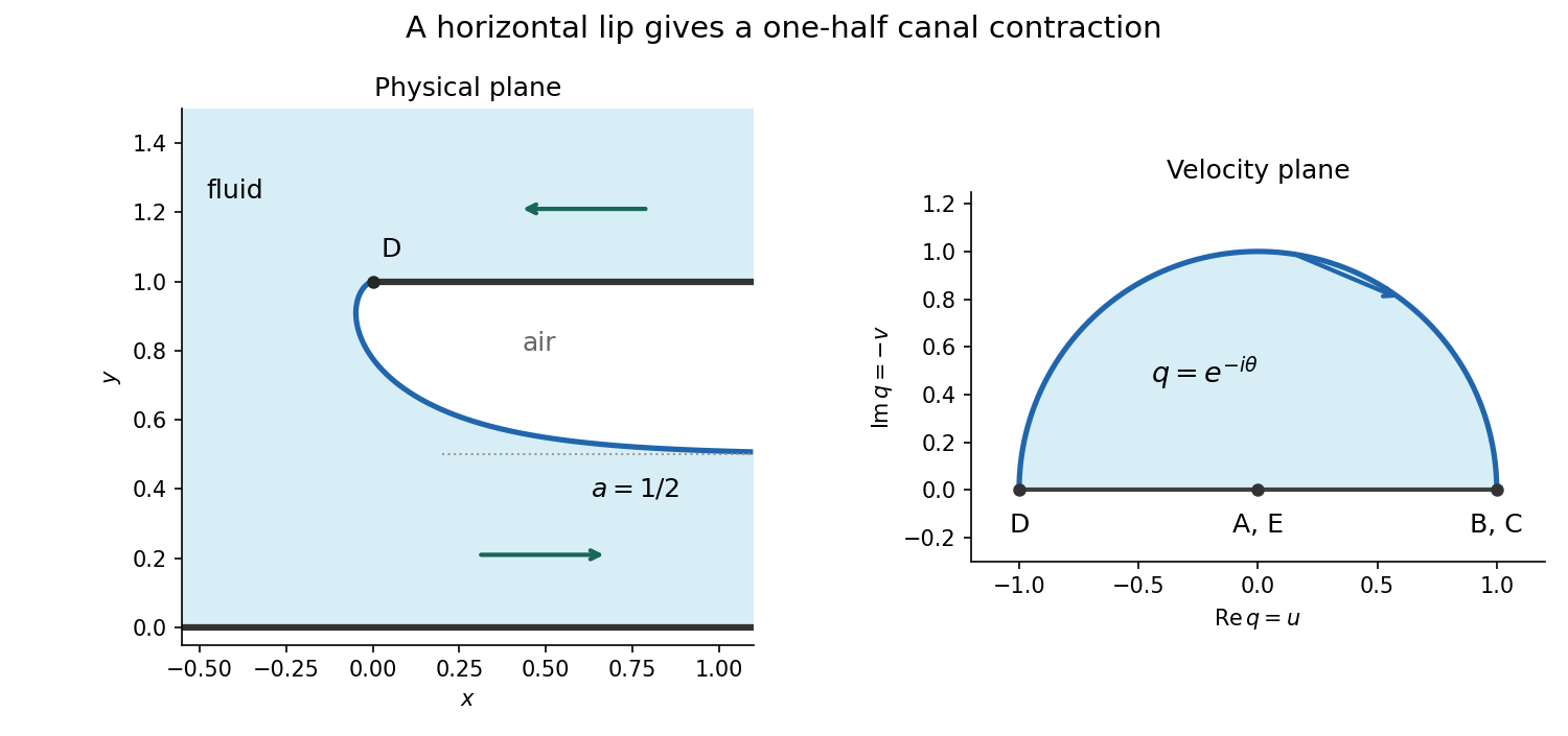
Put . On the floor its values run from zero to one along the positive real axis. Above the plate the flow goes left toward the lip, so the plate velocities run along the negative real axis from zero at to at . On the fluid free boundary Bernoulli's equation and its constant pressure give . Its downward velocity has , hence . Consequently the hodograph plane domain isthe upper unit semicircle. Its marked boundary values are , , and .
For the velocity potential strip, maps to the upper half-plane. The real Möbius transformationpreserves that half-plane and sends its marked endpoints to in the order .
For the hodograph plane, first put . Its image is the second quadrant, bounded by the negative real ray and positive imaginary ray. Squaring takes that quadrant to the lower half-plane, and negating restores the upper half-plane. Thushas exactly the same three marked values. Uniqueness of a conformal map to a half-plane with three assigned boundary values makes these maps equal. Cancel the minus signs to obtainThe sign in the intermediate map is important for identifying the upper, rather than lower, half-plane.
On the fluid free boundary write , with : the lip has and the downstream limit has . ThenSubstitution into the relation from part (ii) givesThe surface lies on the top of the velocity potential strip, so its logarithm has imaginary part , givingFinally , and thereforeThe source's typeset is interpreted as , as the derivation requires.
Integrate real and imaginary parts from the lip value :The identities andgive the explicit parametrizationAs , and . This must be the downstream height , soThe surface initially moves slightly left of the lip before turning right. Its leftmost point occurs at , with . This is the half-contraction free streamline at a horizontal canal lip.
Orient and label its left side plus and its right side minus. Assume the density is Hölder continuity near the point in question, or has sufficient regularity for the boundary limits below. The source does not explicitly state this regularity assumption. Parametrize locally by oriented arclength , with . Define the Cauchy principal value by removing equal arclengths on the two sides:Subtract from the numerator near . The Hölder continuity remainder is locally bounded in absolute value by a constant times for some , so its integral has the same limit from the two sides. The constant part contributes half the residue, with sign determined by the side of the small semicircle. This proves the Sokhotski–Plemelj theoremIn particular and the Cauchy principal value term with coefficient equals . Substituting these two identities into the singular integral equation gives
Choose a canonical homogeneous solution whose boundary values do not vanish, and account for any permitted zeros or poles when forming a quotient. The assumptions alone do not ensure that an arbitrary homogeneous solution has this property. Its jump relation isDividing the inhomogeneous relation by therefore givesThe Cauchy integral solves this additive jump. More generally every solution in the chosen analytic class haswhere has no jump across and obeys the applicable growth, endpoint and divisor conditions. Setting gives exactly the intermediate formula printed in the source.
Let . Applying Sokhotski–Plemelj theorem to the displayed solution and subtracting boundary values yieldsUseThe normalized particular solution is consequentlyand the full solution isThus the printed expression is a particular solution; homogeneous terms need separate normalization. To see why “general” cannot hold without qualification, take the positively oriented unit circle, , , and . Then and are nonzero on the contour. The analytic pair , satisfies the homogeneous jump and decays on the exterior side. Its nonzero density has these very Cauchy boundary values and solves the original homogeneous equation, whereas the source formula with gives zero. This is homogeneous freedom in a scalar singular integral equation; endpoint and index conditions determine which jump-free additions are permitted.
The two holomorphic function functions agree throughout their overlap region strip, so they define a single holomorphic function on the union of their domains, which is the whole complex plane. The resulting entire function is bounded outside a sufficiently large disk by the assumptions at infinity. It is bounded on the disk by continuity and compactness. Liouville theorem therefore makes it constant:Agreement on an open overlap region is what permits analytic continuation; equality of unspecified boundary values alone would need additional hypotheses.
First state the normalization needed for the displayed logarithmic factorization: choose a continuous holomorphic function branch in the strip that tends to zero at both horizontal ends and has sufficient decay for its Cauchy integrals. In particular the index of the kernel along a horizontal line must be zero.
Choose and let , both oriented from left to right. PutThe first is analytic above the lower line and the second below the upper line. On the region between the lines, closing a rectangle gives : the lower horizontal side is traversed forward and the upper side backward. HenceThe equation becomes on the overlap region. With the canonical bounded factors normalized at infinity, these two products glue to a bounded entire function. Part (a) givesThis is Wiener-Hopf factorization with the quotient convention used in this question.
The source hypotheses require a qualification: nonvanishing in the strip and do not by themselves force index zero or a logarithm tending to zero at both ends. For exampleis analytic and nonzero for , tends to one at both ends, but winds once around zero along the real line. A logarithm continued along that line changes by , so it cannot have the stated normalization at both ends. One must first separate the index factor, or allow appropriately subtracted factors and a correspondingly different common-function growth class. The displayed constant conclusion follows under the canonical zero-index assumptions above; it is not an unconditional consequence of the two printed properties of . This is the issue measured by the Index of a Wiener-Hopf kernel.
Use the same normalized factors and contours as in part (b), and put . Multiplying the inhomogeneous equation by givesThe additive Cauchy decomposition has on the overlap region. Subtract it from this equation:Under the same convergence and boundedness assumptions, these expressions are analytic on complementary half-planes, agree on their overlap region, and glue to a bounded entire function. ThusIf the decay is too weak for an unsubtracted Cauchy integral, the subtraction and resulting common-function growth condition must be specified. Merely asserting pointwise is not a substitute for the needed integral transform convergence.
For , put , so . The Laplace transform for the Gamma function, analytically continued from positive real , givesChoose in the upper half-plane. Since ,This integral is absolutely convergent throughout the upper half-plane. On the nonzero real axis it converges conditionally by Dirichlet test for improper integrals, and its value is the upper boundary limit of the same branch. In particular negative real has argument , not in this formula.
At the integral diverges at infinity; in the lower half-plane its exponential function factor grows and the ordinary improper integral diverges. The origin itself causes no local-integrability problem for . A useful continuation of the chosen power uses a branch cut descending from with argument in .
Use the Fourier transform convention , initially in a class where the integral transforms and subsequent limits are defined. Transforming Laplace's equation gives on real . Decay for selectsThe boundary trace is the sum of its negative-half-line unknown and the given positive-half-line datum. The normal derivative is zero on the negative side. ThereforeFor the convention, negative support gives a integral transform analytic for , and positive support gives one analytic for , subject to the appropriate endpoint interpretation. The normal trace in this particular problem requires a finite-part interpretation, detailed below.
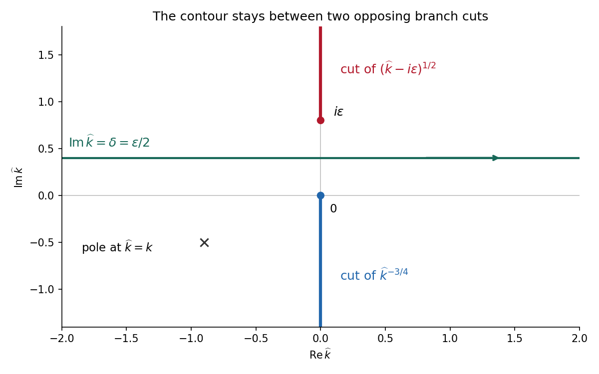
For the Wiener-Hopf method, regularize the real-axis kernel byTake the branch cut of vertically downward from and that of vertically upward from . Their product on the real axis is the positive square root . The branch of has its cut downward from zero. Dividing the regularized equation by givesThe forcing is analytic in , between its two cuts. Decompose by Cauchy integrals on two horizontal lines within that strip. Separation giveswhen the endpoint growth class makes the common entire remainder bounded. For one can take the minus Cauchy integral on , with , obtainingThe integrand is at infinity, so the Cauchy integral converges there. In the limit choose , for example ; a fixed positive cannot remain between zero and . With denoting the limiting lower-analytic branch and with the prescribed limiting interpretation,The numerator square root has a cut going upward from ; the power has a cut going downward from zero. The contour passes between them. The pole is below this contour when is in the lower integral transform domain. These branch choices are essential, rather than independent principal powers of the factors.


There is an important mathematical limitation in the source's ordinary integral definition of . An explicit harmonic function particular solution in polar coordinates isEach separated polar power is harmonic function; at it has the required Dirichlet boundary condition value, and at its angular derivative vanishes, giving the required zero normal derivative. It also decays at infinity. Its unknown boundary traces areThe last function is not locally integrable at zero. Therefore the printed ordinary integral diverges, even for . The integral transform calculation is valid for this solution only after specifying a Hadamard finite-part integral, or equivalently a distribution boundary trace.
For the canonical homogeneous extension of this power, the two transformed traces areThe first is analytic below and the second above. The second formula follows from and the finite-part continuation of the Laplace transform. Substituting their real-axis boundary values directly verifies the boxed integral transform relation for both signs of , so the qualification can be checked without relying only on formal factorization.
There is also homogeneous corner freedom:satisfies zero Dirichlet boundary condition data on the positive axis, zero Neumann boundary condition data on the negative axis and decay at infinity. Its negative trace has integral transform , corresponding to the term . Higher singular modes would also satisfy the homogeneous boundary conditions for integers , but are excluded if the negative trace is required to be locally integrable. Thus the one-constant formula belongs to a specified corner-growth class. The original boundary conditions alone, without that class, do not assert uniqueness. These facts form the finite-part normal trace for mixed quarter-power boundary data.
Articles by others on the same topic
There are currently no matching articles.