Past exam of the physics A course of the University of Cambridge / 2010 / Paper 1 / Section B

Measure both vertical displacements upward from static equilibrium, so gravity cancels. The spring force changes by $k(x_1-x)$, while the damper is attached to a fixed surface and supplies $-b\dot{x}$. Newton's second law givesFor sinusoidal steady motion, substitution of $x=\mathrm{Re}(RA{e}^{i\omega t})$ gives the spring-base displacement response with a grounded damperA decaying homogeneous transient must be added unless initial conditions already select steady state. At low frequency, $R\to 1$ and the mass follows the slowly moving support; the first correction is $-ib\omega /k$. At high frequency, $R\sim -k/(m{\omega }^2)$: inertia suppresses motion and reverses its phase relative to the support. There is no $ib\omega$ in the numerator because the damper's other end does not move.

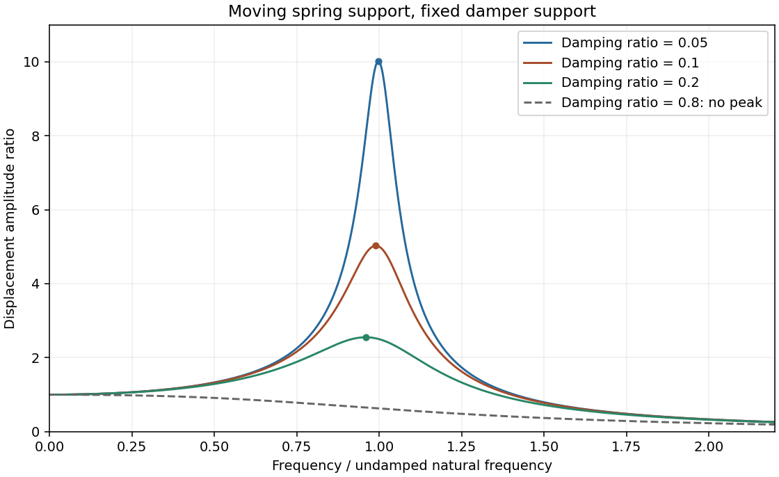
Minimize the squared denominator $D=(k-m{\omega }^2{)}^2+b^2{\omega }^2$. Its derivative is $2\omega [2m^2{\omega }^2-2mk+b^2]$, givingWrite ${\omega }_0=\sqrt{k/m}$ and $\zeta =b/(2m{\omega }_0)$. Then $|R|=[(1-r^2{)}^2+4{\zeta }^2{r}^2{]}^{-1/2}$ with $r=\omega /{\omega }_0$, and the finite-frequency peak is $1/[2\zeta \sqrt{1-{\zeta }^2}]$. Increasing light damping lowers and broadens the peak and shifts it left; the low-frequency limit remains1 and the high-frequency decay remains proportional to ${\omega }^{-2}$.

The resonance versus oscillatory damping thresholds differ. For $b^2\ge 2mk$, the maximum is at zero frequency and the curve decreases monotonically. This threshold is $\zeta =1/\sqrt{2}$, distinct from the free-oscillation critical damping threshold $\zeta =1$.

A dispersive wave has phase speed depending on frequency. Its phase velocity is $v_p=\omega /k$, whereas the group velocity $v_g=d\omega /dk$ describes a narrow wave packet in a lossless single branch. Examples are deep-water gravity waves, ${\omega }^2=gk$, and electromagnetic waves in a cold plasma, ${\omega }^2={\omega }_p^2+c^2{k}^2$.

The fixed-edge membrane waveguide has transverse profiles $\sin (n\pi y/b)$ withThere is no nonzero n=0 displacement satisfying both fixed-edge conditions. Even though the unconfined membrane is nondispersive, transverse confinement makes propagation along x dispersive. The membrane-guide phase and energy speeds are, for a propagating mode,For positive $k_x$, the phase speed exceeds v while group speed is below v. At cutoff $k_x=0$ the formal phase speed diverges, but group speed vanishes; no finite longitudinal energy flux is implied.

With the supplied width and speed, $f_{c,n}=10n\mathrm{kHz}$. At15kHz only n=1 propagates:The negative value represents travel in the opposite direction; higher transverse modes are evanescent.

At5kHz every transverse mode is below cutoff, so no propagating guided mode exists. A driven boundary can produce an evanescent near field. For n=1 the decay coefficient is $\sqrt{(20\pi {)}^2-(10\pi {)}^2}=10\pi \sqrt{3}=54.4{\mathrm{m}}^{-1}$, an e-folding distance of18.4mm. This is decay along the guide, not attenuation of an otherwise propagating lossless wave.

At25kHz, the n=1 and n=2 modes can propagate, withThey have different phase and group speeds, so a launch exciting both produces multimode propagation and possible beating. Actual mode amplitudes depend on the transverse launch profile; their existence does not guarantee both are excited. Modes n≥3 remain evanescent.

In Fraunhofer diffraction, the phase difference from aperture coordinate y to observation angle theta is $qy$, with $q=2\pi \sin \theta /\lambda$. Coherent superposition of the transmitted field elements therefore givesThe common propagation factor is omitted. This is the Fourier transform of the complex amplitude transmission, not of its intensity.

For a uniform slit of total width $W=0.2\mathrm{mm}$, integration gives ${\psi }_0=W\mathrm{sinc}(qW/2)$, where $\mathrm{sinc}s=\sin s/s$. Its normalized intensity is ${\mathrm{sinc}}^2(\pi W\sin \theta /\lambda )$, with a central maximum and first zeros at $\sin \theta =\pm \lambda /W=\pm 0.0025$.

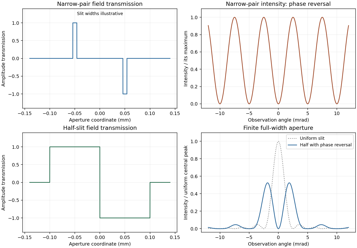
For a half-covered slit choose $T=+1$ on the left half and $T=-1$ on the right. Put $h=W/2$ and $s=qh/2$. The two equal rectangles have centres separated by h, soThis half-slit phase-step diffraction factorization is the phase-reversed two-slit interference factor multiplied by the diffraction envelope of each half-slit. Here the half-slit width and centre separation both equal the earlier0.1mm separation. The central intensity is zero; the largest off-axis pair satisfies $\tan s=2s$, giving $|\sin \theta |\simeq 0.00186$. Other zeros are at $s=m\pi$. The plot includes the requested uniform-slit and half-covered patterns.

The slit transmissions have the same magnitude but opposite phase. An ideal narrow-slit representation isEquivalently draw two narrow rectangles at $y=\pm d/2$, one at+1 and the other at−1, and zero elsewhere. A finite rectangle width gives each slit its own diffraction envelope. The original aperture plot shows such rectangles with explicitly illustrative width; the negative value is a field phase reversal, not negative transmitted intensity.

For the narrow pair, the amplitude is $e^{-iqd/2}-e^{iqd/2}=-2i\sin (qd/2)$. Hence phase-reversed double-slit diffraction givesThere is a central dark fringe. Minima obey $d\sin \theta =m\lambda$, maxima $d\sin \theta =(m+1/2)\lambda$, and the near-axis angular fringe period is $\lambda /d=0.005\mathrm{rad}$. Finite slit widths multiply this interference profile by their single-slit envelope. The parent plot includes the narrow-pair profile.

Fresnel diffraction retains the quadratic transverse propagation phase; Fraunhofer diffraction neglects it and leaves an aperture Fourier transform. Expanding the propagation distance gives $z+y^2/(2z)+\cdots$. The aperture phase variation is of order $\pi {\rho }^2/(\lambda z)$, so the crossover scale is $z\sim {\rho }^2/\lambda$, with far-field propagation requiring a much smaller Fresnel number than1.

Here $\lambda \simeq 0.0100\mathrm{m}$ and the full gap width gives ${\rho }^2/\lambda =25\mathrm{m}$, comparable with the16m range. More decisively, measured from the grazing line of sight to the far gap edge, the quadratic phase reaches $\pi (0.5{)}^2/(0.01\times 16)=4.91\mathrm{rad}$. Fresnel diffraction is required; conventions using a half-width change the quoted Fresnel number but not this phase test.

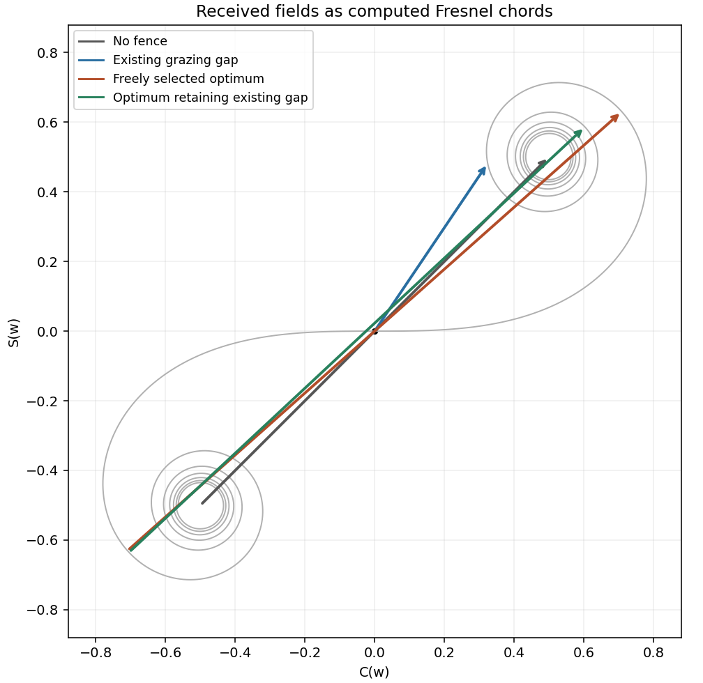
Define $F(w)=C(w)+iS(w)$ with the normalization in the paper. The grazing-edge gap spans $w=0$ toThe Cornu chord power normalization uses a received field proportional to $F(w_g)-F(0)$, while no fence gives $F(\infty )-F(-\infty )=1+i$. Numerical Fresnel integration gives $C(w_g)=0.3245$, $S(w_g)=0.4818$, and thereforeThe two labelled child answers specify the corresponding vectors.

For the largest contiguous Fresnel aperture, a freely chosen single contiguous opening must maximize the chord between two points of the Cornu spiral. Its longest chord joins $F(-w_{\ast })$ to $F(w_{\ast })$, where the first maximum radius satisfies $C(w_{\ast })\cos (\pi w_{\ast }^2/2)+S(w_{\ast })\sin (\pi w_{\ast }^2/2)=0$. This gives $w_{\ast }=1.2094$ andHere x is signed displacement along the fence from the grazing optical axis. The pointwise Fresnel gain versus integrated transmitted power distinction explains why an aperture can concentrate more power at one receiver than the fully open field through constructive interference; this is not an increase of integrated transmitted power.

The existing-opening constraint in Fresnel aperture optimization matters literally: the original gap already occupies $[0,0.5]\mathrm{m}$. The symmetric optimum would require filling its far end. If only further removal is permitted and the final opening must be connected, maximize the chord subject to $w_{-}\le 0$ and $w_{+}\ge 1.768$. The constrained optimum is approximatelyThese are different optimization assumptions; both are stated so the original gap is not silently replaced. The model treats the fence as an ideal opaque screen and ignores ground reflections or additional propagation paths. ^[ref]

The grazing-gap signal is the chord from $F(0)=0$ to $F(1.768)$, approximately $(0.3245,0.4818)$ in the (C,S) plane. Its squared length determines received power after applying the same propagation normalization used for the open field. Reversing which gap edge grazes the ray reflects both limits and leaves the power unchanged.

With the whole fence removed, the vector joins $F(-\infty )=(-1/2,-1/2)$ to $F(+\infty )=(1/2,1/2)$. It is $(1,1)$, with squared length2. The normalized power ratio must compare the gap chord to this full chord, not to the half-plane chord from the origin to one limiting point.