spin normalization in two-dimensional free-electron state counting. Treat the mobile electrons as independent particles in a constant interior potential, with parabolic dispersion , and impose confinement or periodic boundary conditions. electron–electron interactions and the detailed periodic ionic potential are neglected, while Fermi statistics are retained. Each spatial state occupies area in two-dimensional wavevector space. For spin degeneracy ,The printed coefficient is the per-spin density of states. Unpolarized spin-one-half electrons have , doubling it. Actual graphene near its Dirac points has approximately linear dispersion, so its energy-dependent density of states is not this parabolic-model result; the plane geometry alone does not establish the free-electron dispersion.[ref]
Two-Dimensional Gas of Massless Dirac Fermions in Graphene by Konstantin Novoselov and others. Abstract: massless Dirac charge carriers rather than a finite-mass parabolic band
Occupied disk and Fermi energy. At zero temperature fill the lowest states up to a disk of radius . State counting givesThus the physical spin-degenerate result is . If instead counts one spin species, the per-spin convention gives . Each occupied wavevector can contain one electron of each allowed spin, never two in the same complete one-particle state.
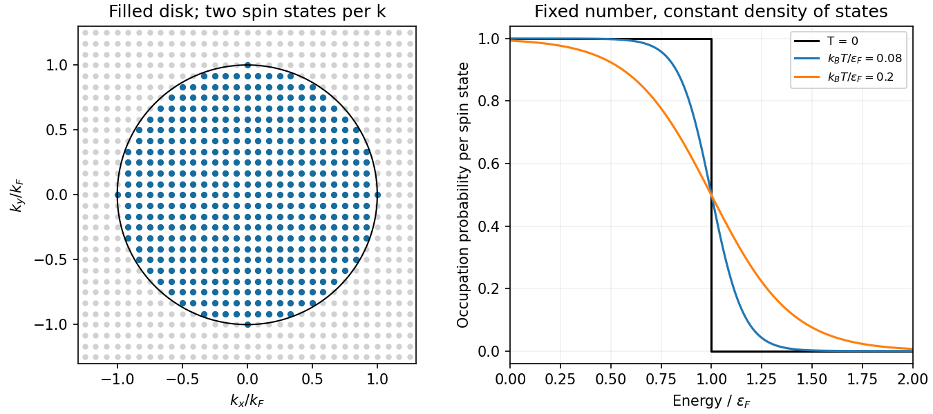
Original occupied wavevector disk and Fermi-Dirac occupations for a parabolic two-dimensional electron gas
. Details. 
Occupation probability and chemical potential of a two-dimensional ideal Fermi gas. A single fermion state permits occupation zero or one. In a grand canonical ensemble their relative weights are and . Normalizing givesThe chemical potential is fixed by the total particle number. Here the total density of states is constant above the band bottom. Integrating the occupation gives , and thereforeThe approach is exponentially close in this ideal two-dimensional constant-density-of-states model; a three-dimensional correction should not be inserted here. A narrow interval of width of order around is thermally smeared.
One mass per cell. If is the displacement from equilibrium, the two springs give . Substituting yieldsThe first Brillouin zone is ; adding leaves the sampled displacements unchanged. The branch is linear near zero, with sound speed , and reaches at either zone edge.
Two masses per cell. Take a cell of length , with light displacement and heavy displacement . The coupled equations reduce toA nonzero displacement requires determinant zero:Solving this quadratic in givesNow the first zone is . The minus branch is acoustic: as , both sublattices move together and . Its sound speed is . The plus branch is optical: at the atoms move oppositely with , giving finite frequency . This terminology describes relative motion; optical activity itself also requires coupling to the electromagnetic field.
diatomic-chain zone-edge polarizations and dimensionality. At the edge, , so the heavy and light sublattices decouple: the acoustic edge frequency is and the optical edge frequency is . HenceThe acoustic edge mode moves only the heavy sublattice; the optical edge mode only the light one. If , the gap closes and the two branches are the zone-folded monatomic branch.
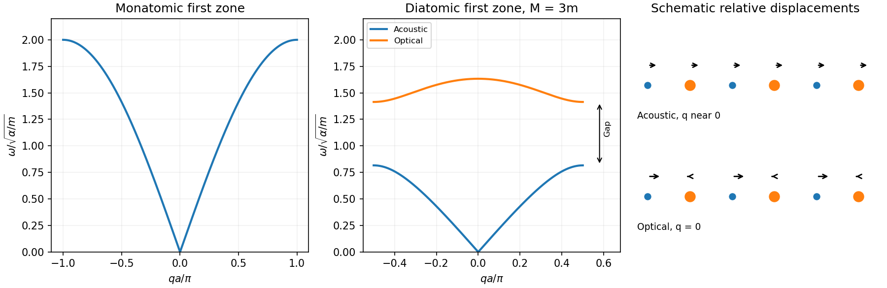
Original monatomic and diatomic chain dispersions, zone-edge gap and long-wavelength displacement patterns
. Details. 
A three-dimensional crystal with two atoms per primitive cell has six branches: three acoustic and three optical. For propagation along a suitable symmetry direction these resolve into one longitudinal and two transverse branches of each type. The wavevector and Brillouin zone are three-dimensional; anisotropic force constants determine the dispersions, and polar crystals can have longitudinal–transverse optical splitting. A universal six-branch curve cannot be specified from masses alone.
Articles by others on the same topic
There are currently no matching articles.