The original diagram places hard walls at and , and the central plateau on is exactly at the indicated ground-state energy. This equality determines the middle of the requested sketch. In the Time-independent Schrödinger equation,the central interval has , hence . The ground state can be chosen real and positive inside the walls by the nodeless theorem for a one-dimensional ground state. Reflection symmetry makes it even about , so its linear central segment must be constant.
The hard-wall boundary conditions are . On both outer intervals , so the positive wavefunction has negative curvature and is sinusoidal. Wavefunction matching at a finite potential step requires both and to remain continuous at ; the derivative therefore vanishes where each sinusoidal flank meets the flat middle. A normalized representative isEach side contributes and the plateau contributes to the squared norm before multiplying by . The corresponding consistency condition is ; a numerical energy is not required for the sketch.
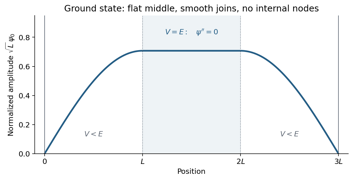
The positive ground-state wavefunction has sinusoidal flanks and a flat central segment at V equals E
. Details. Thus the ground state at the top of a central rectangular barrier has no internal nodes, continuous value and slope, and a flat middle, rather than an exponential dip through a classically forbidden region. Multiplication by an overall constant phase changes none of these physical features.
Use the canonical commutation relation on a common invariant domain of the operator products. Write , so . Associativity then giveswhereasThereforeAs a direct position-representation check, the momentum operator is . Acting on a smooth function givesThis is the equality of two quadratic position-momentum orderings; it does not make arbitrary rearrangements of noncommuting linear operators interchangeable.
For addition of angular momentum, the allowed total quantum number runs in unit steps from to . With and ,Thus the complete list of multiplets isThe total angular momentum operator has squared magnitude eigenvalue and chosen-axis component eigenvalue . The number of states is , matching the uncoupled dimension .
Use an inverting operational amplifier. Ground the non-inverting input, connect the source to the inverting input through , and connect from the output back to that same input.
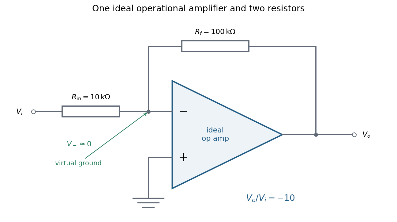


In linear operation the ideal operational amplifier draws no input electric current, and feedback holds the inverting input at the same electric potential as the grounded non-inverting input. This node is a virtual ground. Kirchhoff's current law there givesThe source supplies current , so its input impedance is . The required design is thereforeOnly these two resistors and the single ideal operational amplifier are needed in the signal circuit; its power supplies are implicit. The result assumes an input small enough to keep the output within its linear operating range.
Use the sample mean to estimate each magnetic susceptibility, and the unbiased sample variance with denominator to estimate the repeatability of individual readings. In the numerical scale supplied by the paper,If the repeated measurements have independent random errors, their mean estimates have standard errorsThe difference and its estimated standard uncertainty are thereforeThe separation is about standard errors. Under an approximately normal distribution model with no experimenter-dependent bias, Welch's t-test gives about statistical degrees of freedom and a two-sided p-value of . Thus there is modest evidence against equal underlying susceptibilities at a conventional significance level; overlap of the ranges of individual readings is not an adequate comparison of the means. Five readings per sample provide limited information about the error distribution.
Crucially, material and student exhibit complete confounding: each student measured only one sample. An experimenter-dependent systematic error could mimic the difference. Paramagnetism also depends on conditions such as temperature, so equal material alone does not guarantee equal readings without controlling those conditions. The defensible physical conclusion is the data suggest a difference, but do not establish different materials. Both students should measure both samples in randomized or alternating order, with calibration and temperature controlled, to separate a sample effect from an operator effect. No unit or scale factor absent from the original table has been invented.
Articles by others on the same topic
There are currently no matching articles.