The original diagram places hard walls at and , and the central plateau on is exactly at the indicated ground-state energy. This equality determines the middle of the requested sketch. In the Time-independent Schrödinger equation,the central interval has , hence . The ground state can be chosen real and positive inside the walls by the nodeless theorem for a one-dimensional ground state. Reflection symmetry makes it even about , so its linear central segment must be constant.
The hard-wall boundary conditions are . On both outer intervals , so the positive wavefunction has negative curvature and is sinusoidal. Wavefunction matching at a finite potential step requires both and to remain continuous at ; the derivative therefore vanishes where each sinusoidal flank meets the flat middle. A normalized representative isEach side contributes and the plateau contributes to the squared norm before multiplying by . The corresponding consistency condition is ; a numerical energy is not required for the sketch.
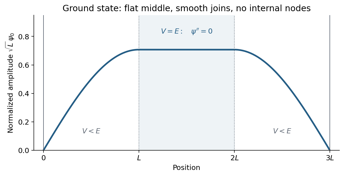
The positive ground-state wavefunction has sinusoidal flanks and a flat central segment at V equals E
. Details. Thus the ground state at the top of a central rectangular barrier has no internal nodes, continuous value and slope, and a flat middle, rather than an exponential dip through a classically forbidden region. Multiplication by an overall constant phase changes none of these physical features.
Use the canonical commutation relation on a common invariant domain of the operator products. Write , so . Associativity then giveswhereasThereforeAs a direct position-representation check, the momentum operator is . Acting on a smooth function givesThis is the equality of two quadratic position-momentum orderings; it does not make arbitrary rearrangements of noncommuting linear operators interchangeable.
For addition of angular momentum, the allowed total quantum number runs in unit steps from to . With and ,Thus the complete list of multiplets isThe total angular momentum operator has squared magnitude eigenvalue and chosen-axis component eigenvalue . The number of states is , matching the uncoupled dimension .
Use an inverting operational amplifier. Ground the non-inverting input, connect the source to the inverting input through , and connect from the output back to that same input.
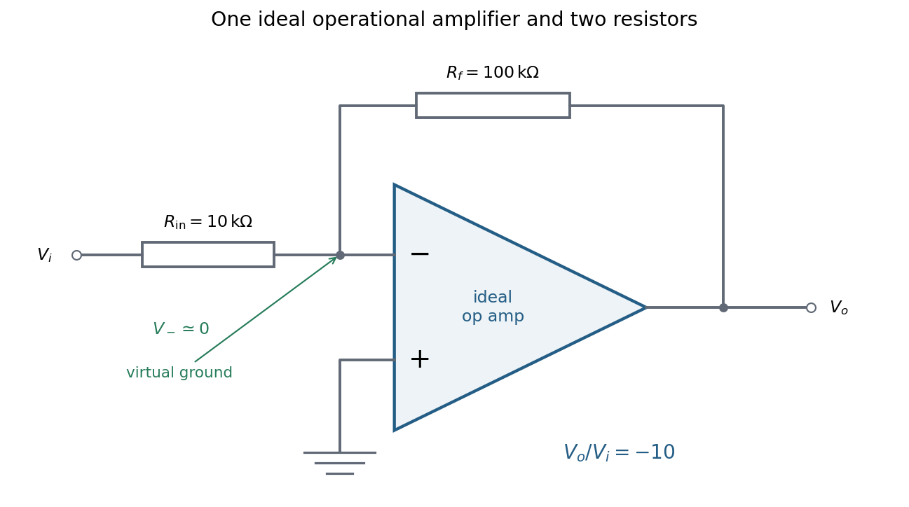
In linear operation the ideal operational amplifier draws no input electric current, and feedback holds the inverting input at the same electric potential as the grounded non-inverting input. This node is a virtual ground. Kirchhoff's current law there givesThe source supplies current , so its input impedance is . The required design is thereforeOnly these two resistors and the single ideal operational amplifier are needed in the signal circuit; its power supplies are implicit. The result assumes an input small enough to keep the output within its linear operating range.
Use the sample mean to estimate each magnetic susceptibility, and the unbiased sample variance with denominator to estimate the repeatability of individual readings. In the numerical scale supplied by the paper,If the repeated measurements have independent random errors, their mean estimates have standard errorsThe difference and its estimated standard uncertainty are thereforeThe separation is about standard errors. Under an approximately normal distribution model with no experimenter-dependent bias, Welch's t-test gives about statistical degrees of freedom and a two-sided p-value of . Thus there is modest evidence against equal underlying susceptibilities at a conventional significance level; overlap of the ranges of individual readings is not an adequate comparison of the means. Five readings per sample provide limited information about the error distribution.
Crucially, material and student exhibit complete confounding: each student measured only one sample. An experimenter-dependent systematic error could mimic the difference. Paramagnetism also depends on conditions such as temperature, so equal material alone does not guarantee equal readings without controlling those conditions. The defensible physical conclusion is the data suggest a difference, but do not establish different materials. Both students should measure both samples in randomized or alternating order, with calibration and temperature controlled, to separate a sample effect from an operator effect. No unit or scale factor absent from the original table has been invented.
Equation and boundary conditions. The delta potential has strength with units of energy times length, because the Dirac delta function has units of inverse length. The Time-independent Schrödinger equation isThe wavefunction is continuous at the origin. A finite jump in would produce a derivative of a Dirac delta function in , with no corresponding term in this potential. A jump in does produce a delta contribution and is allowed. Integrate through a symmetric interval:For continuous finite , the right-hand side vanishes as . ConsequentlyThis derivative jump is the boundary condition associated with the attractive delta potential.
Unique bound state. For , write . Away from the origin, . Normalizability excludes exponentials growing at either infinity, leavingContinuity gives . The derivative jump then becomes . For a nonzero state,There is exactly one positive value of , so exactly one negative-energy bound state. An odd solution would have ; the allowed decaying exponentials would then both vanish identically. Normalize the even solution usingChoosing the overall phase real and positive gives the bound state in a delta potential:It peaks at the origin, has a downward cusp there, and decays exponentially on both sides. Its value, but not its slope, is continuous.
Scattering amplitudes and fluxes. For , put and retain as a strength parameter. A unit-amplitude wave incident from the left hasContinuity gives . The jump condition givesSolving,The probability current of a plane wave of amplitude is in its propagation direction. Since the asymptotic wavenumber is the same on both sides, reflection probability and transmission probability are just and :They satisfy , expressing conserved probability current in this real potential.
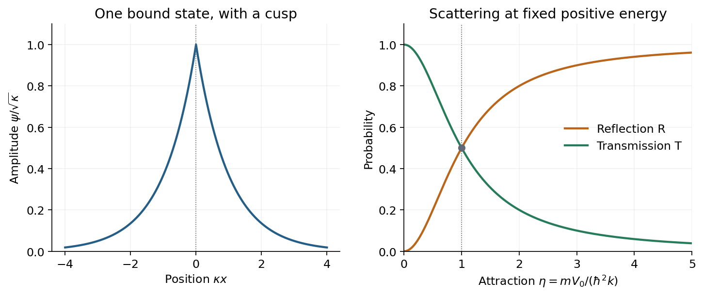
The normalized delta-well bound state and reflection/transmission probabilities as attraction increases
. Details. The right-hand plot uses , proportional to at fixed incident energy. Then rises monotonically from zero to one, while falls from one to zero; they are equal at . Despite the absence of a classical forbidden barrier, an abrupt attractive interaction reflects a quantum wave. Increasing attraction strengthens the derivative mismatch and can approach complete reflection at fixed positive energy. At fixed , increasing incident energy instead makes the well increasingly transparent. The negative-energy bound state and the positive-energy scattering states are different stationary solutions, not an absorptive loss channel.
Hamiltonian and commutators. Use the canonical commutation relation and define . Expanding the product of the given creation and annihilation operators,Therefore the quantum harmonic oscillator Hamiltonian operator isSimilarly,Using gives
Lowering a normalized energy eigenstate. The commutator impliesFor , nondegeneracy of this one-dimensional energy level means . Its norm is fixed by the number operator:Choosing successive eigenstate phases in the conventional way makes , soFor , the same norm is zero, hence . A nonzero lowered ground state would have energy below the lowest allowed level, and positivity of forbids that possibility.
Coherent-state eigenvalue. Applying the annihilation operator term by term, with the contribution zero, givesThusThe coherent state is normalized because . Its annihilation operator is not Hermitian, so the eigenvalue may be complex.
Time evolution. Under the time-independent Hamiltonian operator, each energy component acquires its own phase:Since , the normalization prefactor is unchanged. HenceThe state remains a coherent state, with its complex parameter rotating at the oscillator's angular frequency; the displayed extra factor is a global phase from the zero-point energy.
Reduced radial equation. A spherical harmonic satisfies . Substitute into the Time-independent Schrödinger equation, divide out the angular function, and put . Direct differentiation givesMultiplication by then gives the Radial Schrodinger equationHere is the reduced mass, and the extra positive term is the centrifugal potential.
Boundary conditions. At the origin this finite central potential has no point interaction. The physical radial solution is regular there, requiring ; for , a nonzero constant would give and a point-source singularity of the three-dimensional Laplacian. Mere square integrability alone would not remove that singular solution. For a bound state, the radial probability integral is , so the exterior solution must decay and as .
Solutions for zero orbital angular momentum. For and , defineThe interior equation is ; excludes the cosine. The exterior equation is ; normalizability excludes the growing exponential. ThusThe constants cannot remain independent once the interface is matched. Since the potential step is finite, both and are continuous at :Dividing the equations yields
Existence and number of s-wave bound states. Put , , and . ThenThe lowest branch lies on . Along it, and increases continuously from to infinity. Therefore a first negative-energy solution exists precisely when , orFurther branches begin at as . Hence the bound-state thresholds of a spherical square well give exactly one negative-energy state whenThe upper equality is included: the second branch is then only at , with constant exterior , and is not normalizable. If threshold cases are excluded by convention, the commonly quoted open interval has a strict upper inequality; the physical negative-energy state count at equality is still one.
Deuteron estimate. Using , and gives . At ,The threshold for a second state is , far above the stipulated depth . Thus this model has no radially excited s-wave bound state.
Checking other orbital angular momentum sectors matters before ruling out every excitation. At the first -wave threshold, the regular interior reduced radial function is and the zero-energy exterior function is proportional to . Matching their logarithmic derivatives requires , whose first root is . HenceLarger only increases the centrifugal potential. Therefore no bound orbital excited states are expected in the specified central square-well model. Its spin dependence and tensor nuclear forces have not been specified; the calculation does not resolve the real deuteron's internal spin structure.
Distinguishable noninteracting particles. Interpret as the same external one-particle potential for each particle; the total potential is . The Time-dependent Schrödinger equation isLet and , where . Applying to the product multiplies it by . The time derivative of multiplies it by . Thus the proposed stationary product is a solution providedThe tensor product separates the two independent one-particle dynamics.
Identical spin-one-half particles. Identical fermions require antisymmetry under exchange of the complete position-and-spin labels. First take to be distinct orthonormal spatial orbitals, and defineThe symmetric spatial state must multiply the antisymmetric spin-one-half singlet state; the antisymmetric spatial state must multiply one of the three symmetric spin-one-half triplet states. The four normalized possibilities, each with the common time factor , areThese are the required product states under fermionic exchange symmetry. If , the antisymmetric spatial combination vanishes. Only the product times the singlet remains, as required by the Pauli exclusion principle. A nonorthogonal pair would require different normalization factors; the displayed assumes an orthonormal stationary-state basis.
Weak repulsive Coulomb interaction. For fixed orbitals , first-order perturbation theory gives spatial energy shifts . Here is the direct interaction energy, while the exchange integral for repulsion strength isThe positivity follows from the positive Fourier transform of the Coulomb kernel. Consequently Coulomb exchange splitting of two orbitals givesAll three triplet spin components remain degenerate for a spin-independent Coulomb interaction. Their antisymmetric spatial factor vanishes at coincidence and reduces close encounters. The inequality is strict when ; for negligible orbital overlap, the splitting may vanish. This comparison fixes one particle in each of the specified orbitals and does not rank singlets with a different orbital occupation.
Spin-zero bosons. For one particle in each of the same distinct orthonormal orbitals, the spin factor is symmetric and bosonic exchange symmetry requires . At coincident positions,Thus the bosonic coincidence enhancement in two orthogonal orbitals isThese are joint probability densities, or small-detector-volume limits; an exactly specified point has zero probability in a continuous distribution. If both particles occupy the same orbital, the properly normalized product is already symmetric and the corresponding enhancement relative to distinguishable particles in that same orbital is one. The paper's usual factor-two answer presumes distinct orthogonal input orbitals.
Operators, quantization and rotations. Angular momentum is the generator of spatial rotations. In quantum mechanics, its components are Hermitian operators on their appropriate domains and obeyThese angular momentum commutation relations prevent all three components from having simultaneous sharp values. For example, the Robertson uncertainty principle gives . One conventionally diagonalizes and a selected component :The allowed labels are and . An angular-momentum multiplet has states. The magnitude differs from the largest possible component ; the remaining components fluctuate even in a state with maximal .
The angular momentum lowering operator and its raising counterpart, , satisfyThe ladder terminates at . A rotation through angle about unit vector acts through the unitary operator . Thus quantized components and the continuous rotation of a state are compatible.
Orbital angular momentum. The orbital contribution is associated with motion in space:For a spinless spatial wavefunction, the simultaneous angular eigenfunctions are the spherical harmonics , with and . Single-valued ordinary scalar spatial wavefunctions give integer orbital labels. In a central potential energy, , so stationary states may be labelled by these angular quantum numbers. The angular kinetic contribution appears in the radial equation as , the centrifugal potential. Noncentral interactions need not conserve these orbital labels.
Intrinsic spin and addition. Spin angular momentum is an intrinsic internal degree of freedom with the same commutation algebra. It is not the angular momentum of a small classical charged sphere literally rotating about its centre. For an Electron, and , so in terms of the Pauli matrices. Its squared spin is . Other particles can have integer or half-integer spin, including spin zero.
For one particle with orbital and spin degrees of freedom, ; the two component sets commute with each other. Addition of angular momentum permits . The coupled states are linear combinations of the uncoupled with , determined by Clebsch-Gordan coefficients. A rotationally invariant spin-orbit interaction can conserve while mixing the separate component labels.
Angular momentum also carries a magnetic moment. For an electron's orbital motion and intrinsic spin,The minus signs reflect negative electric charge. With the Bohr magneton , a spin projection has . A magnetic field can therefore distinguish angular-momentum states through their interaction energy .
Stern–Gerlach measurement. In the Stern-Gerlach experiment, atoms emerge from a heated source, pass through collimating apertures, traverse a strongly inhomogeneous magnetic field, and strike a position-sensitive screen. The beam is neutral, so its separation is interpreted through the atomic magnetic moment rather than the ordinary charged-particle Lorentz force. Near a chosen quantization direction, the interaction givesA uniform field can exert a torque but would not separate the beam by this translational force; the gradient is essential. Different allowed magnetic-moment components become correlated with different trajectories. A classical ensemble with continuously varying orientations would yield a continuous spread, whereas discrete quantum components yield separated channels.
In the modern electronic description of ground-state silver, filled shells cancel their electronic angular momenta and the unpaired electron has , , . The effective electronic measurement therefore has two components, approximately , rather than an orbital , which is not allowed. For positive field gradient the electronic component has negative and deflects downward in this coordinate convention. Nuclear spin and hyperfine structure are neglected in this simplified two-channel account. Historically the original splitting preceded the electron-spin interpretation, so the modern explanation should not be confused with the original investigators' interpretation.
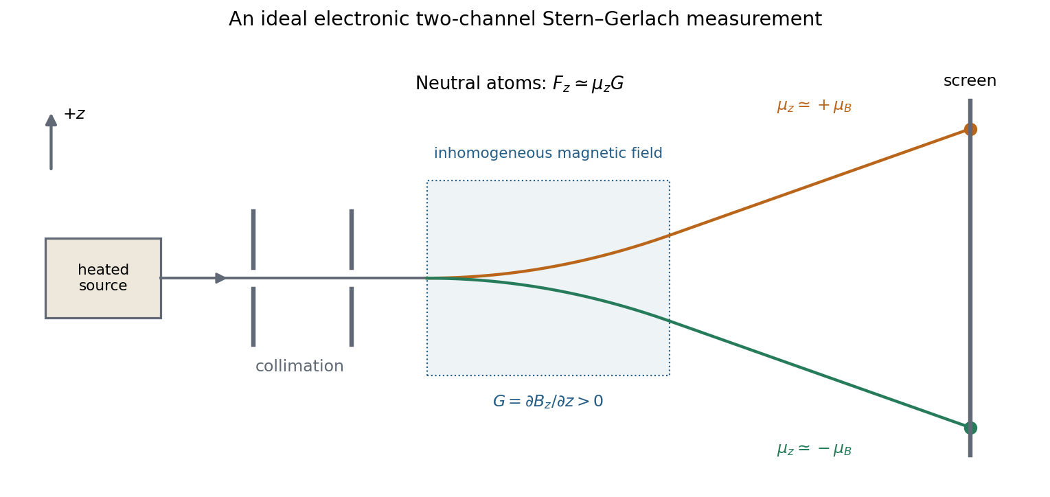


More generally a prepared spin state gives the two outcomes with probabilities . Selecting one channel prepares a state for further measurements. An ideal second analyser along the same axis then gives a definite result, whereas one along a perpendicular axis gives two equally likely outcomes for a spin-one-half eigenstate. This connects the apparatus directly to incompatible spin components and the Born rule. Angular momentum is quantized through its operator algebra; the Stern–Gerlach gradient turns that discrete internal information into spatially distinguishable outcomes.
The Bohr model combines classical circular motion in the Coulomb potential with explicitly quantum postulates. A one-electron atom of nuclear charge has electron–nucleus reduced mass . With , the relative circular orbit obeysBohr postulates permitted nonradiating stationary orbits with , for . These assumptions giveFor hydrogen with the nucleus taken infinitely heavy, the radius is the Bohr radius, . The finite reduced mass gives the small nuclear-motion correction, and increasing contracts the one-electron orbit.
The circular-motion equation gives while the potential energy is , so the total energy is . Substituting the quantized radius yieldsFor the heavy-nucleus hydrogen approximation, . The ionization threshold is zero energy, so removing the ground-state electron requires about .
The model further postulates that radiation is emitted or absorbed only in transitions between stationary orbits, with photon energy . Emission from givesThus it reproduces the principal hydrogen spectral series, their limiting wavelengths, and the gross hydrogenic energy levels. For example, in hydrogen has and , a visible line. Absorption reverses the transition when the photon matches the energy gap.
The achievement is that quantized energies explain discrete spectra, but the model's stationary orbits are postulates rather than consequences of classical electrodynamics: an accelerating classical charge would radiate. It does not provide a general calculation of line intensities or transition selection rules and fails as a quantitative theory of many-electron atoms. Spin, fine structure and the full Zeeman effect require further physics. Modern quantum mechanics replaces definite electron orbits by wavefunctions and quantum probabilities. In particular, the true hydrogen ground state has , so its orbital angular momentum vanishes; the model's rule should not be identified with the modern orbital eigenvalue rule . Bohr's energy quantization remains a successful hydrogenic approximation, while its literal orbital picture does not.
Ehrenfest theorem relates the dynamics of quantum expectation values to operator commutators. For a normalized state obeying and a possibly time-dependent observable , differentiate . Using the adjoint Schrödinger equation for the bra givesThusThe identity assumes a common domain on which the required products and derivatives are defined.
For , the canonical commutation relation gives and . ThereforeThese resemble Hamilton's equations and Newton's second law, but generally . If the state is localized about , a local expansion givesThe classical trajectory equation for the mean is accurate when the force changes little across the wave packet. For a quadratic harmonic potential, is linear and this closure is exact for every state with the relevant finite moments: . This exact classical evolution of the centroid does not eliminate its quantum position uncertainty or make every state a point particle.
The correspondence principle is broader: quantum predictions recover classical ones in an appropriate limit, such as large action compared with and observations that cannot resolve individual quantum levels. It is not the assertion that every large quantum number automatically makes every possible state classical. Delocalized superpositions and interference can remain significant unless the physical preparation and measurement justify a classical description.
A spectral example is useful. For a quantum harmonic oscillator, neighboring levels differ by , giving transition frequency , equal to its classical oscillation frequency. A coherent state makes the connection more concrete: its mean position and momentum oscillate classically while the finite-width Gaussian profile retains its quantum uncertainty. For hydrogenic Bohr levels , transitions between nearby large have , which equals the classical circular orbital angular frequency in that model. Ehrenfest's theorem supplies an exact expectation-value bridge; a classical trajectory follows only when the force can also be evaluated at the mean position.
A Hermitian operator satisfies the adjoint symmetry conditionfor vectors in its specified domain. For a finite matrix this means . For an unbounded differential operator, boundary conditions and domains matter: symmetry on a chosen domain is not alone sufficient for self-adjointness. Physical observables require the corresponding self-adjoint operator and its spectral measure. This distinction prevents purely formal integration by parts from being mistaken for a complete operator definition.
Real eigenvalues. If with nonzero norm, Hermiticity impliesso . Thus eigenvalues representing measurement outcomes are real.
Orthogonality. For eigenvectors ,Hence , and distinct eigenvalues have orthogonal eigenvectors. Within a degenerate eigenspace, Gram-Schmidt orthogonalization can choose an orthonormal basis. In finite dimensions the spectral theorem gives a complete orthonormal eigenbasis andwhere projects onto each eigenspace. In infinite dimensions a continuous spectrum may require a spectral integral rather than a normalizable eigenvector for every possible outcome; a position operator on the full line is a familiar example.
Measurements and probabilities. In the discrete case the Born rule assigns probability to the outcome . For a nondegenerate eigenbasis, gives probabilities , withThe variance vanishes precisely when the state lies in an eigenspace with a single sharp outcome. A repeatable ideal projective measurement prepares the corresponding eigenspace; superpositions of different eigenvalues do not have a preassigned sharp value of that observable in this description.
Compatibility and dynamics. Commuting Hermitian matrices admit simultaneous diagonalization, permitting a common set of sharp labels. For example commute, whereas do not. In the differential-operator setting the corresponding spectral compatibility requires appropriate domain conditions. Noncommuting observables obey the Robertson uncertainty principleThe canonical commutation relation then gives .
The Hamiltonian operator represents energy. A self-adjoint generates unitary time evolution, , preserving norm and total probability; its eigenvalues determine stationary-state phases and transition energies. Hermiticity supplies real outcomes and orthogonal eigenspaces, while self-adjointness and the spectral theorem make these measurement and evolution rules mathematically complete.
Ideal spectrum. Write , with . The overdamped harmonic-trap power spectrum is a Lorentzian line shape:Thus its log-log plot is horizontal at low frequency and approaches slope at high frequency, changing around . The left panel below compares two characteristic frequencies with the same illustrative ; a common numerator is explicitly assumed for this sketch. Their high-frequency tails coincide and their low-frequency plateaux differ as .
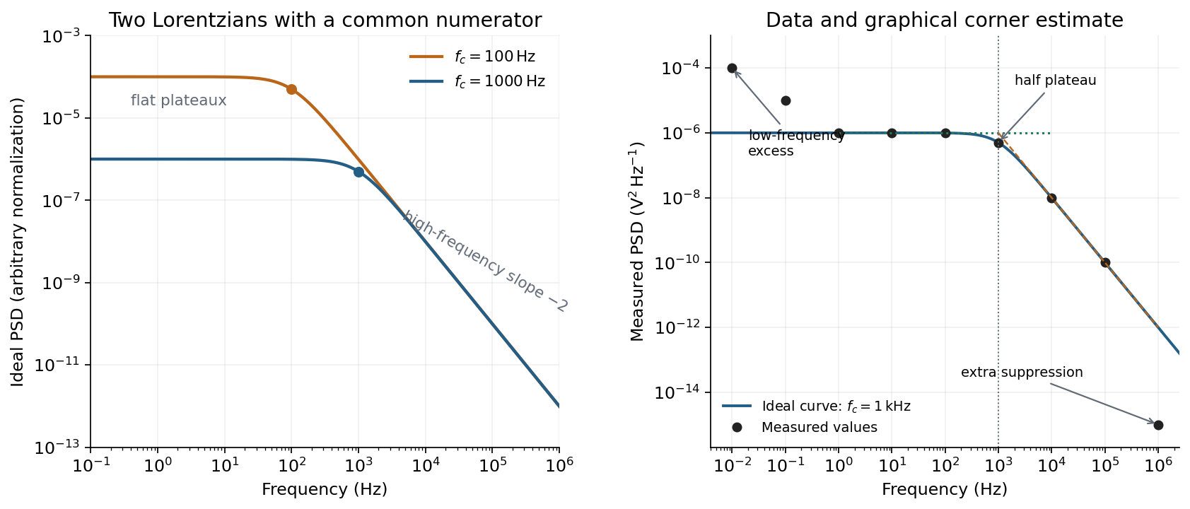
Ideal Lorentzian spectra at two corner frequencies and the measured spectrum with its graphical corner estimate
. Details. 
The right panel plots all nine original data points, including the very-low-frequency excess and the highest-frequency suppression. It also shows the ideal curve inferred only from the requested intermediate range.
Graphical corner estimate. Between roughly and the measured power spectral density is approximately the plateau . At and ,so the descending asymptote is with . The graphical corner frequency of a Lorentzian spectrum is where these asymptotes intersect:Independently, the measured value is exactly the half-plateau condition . Both graphical readings agree. The inferred ideal curve is approximately
Low-frequency excess and recording duration. The two lowest-frequency measurements increase approximately as , whereas the ideal trapped oscillator tends to a constant plateau. This resembles flicker noise or slow apparatus drift superposed on the motion. The transimpedance amplifier, detector or environment could contribute; the spectrum alone does not identify the source uniquely. It would be incorrect to attribute that whole excess to the ideal Brownian oscillator.
A finite record of duration has ordinary Fourier frequency resolution of order . Resolving the lowest tabulated frequency therefore requires at leastThis is a formal lower bound corresponding to about one cycle; a reliable noise-spectrum estimate normally needs a substantially longer record and averaging.
Sampling. The largest reported frequency is . The Nyquist–Shannon sampling theorem therefore gives the Nyquist lower boundIn practice choose a rate above , with an analogue anti-aliasing filter suppressing unmeasured content above half the sampling rate. Exact equality cannot recover an arbitrary pure sinusoid precisely at the boundary for every phase; it is the limiting lower-bound answer rather than a comfortable practical sampling design.
High-frequency departure and amplifier design. Extrapolating the fitted tail to predicts approximately , while the measured value is . The observed drop from to has effective logarithmic slope , much steeper than the ideal .
A detector or amplifier bandwidth limit, or intentional filtering before digitization, can explain such suppression. For a linear filter the spectral density transformation under a linear filter is , so the last point corresponds approximately to an additional relative voltage gain , if attributed entirely to the readout transfer function. One additional point does not determine a unique filter order or identify the circuit responsible.
Rolling off an amplifier's gain beyond the useful signal band reduces integrated high-frequency noise, suppresses interference, and helps prevent aliasing in the analogue-to-digital converter. Limiting high-frequency loop gain can also improve feedback stability and suppress unwanted oscillation. The cutoff must retain the frequencies needed for the measurement; excessive filtering would distort the desired fluctuation spectrum itself.
Electrical noise reduction starts by identifying what is unwanted in the measured signal and where it enters. Increasing gain amplifies both signal and input noise; it does not by itself improve the input signal-to-noise ratio. Separate intrinsic component fluctuations, amplifier noise and external pickup before choosing a remedy.
Physical sources. A resistor at temperature has classical one-sided open-circuit thermal electrical noise density per hertz. In a flat measurement bandwidth , its rms voltage is . Lowering an appropriate resistance, reducing temperature or narrowing the useful bandwidth can reduce this noise, with loading and signal-gain tradeoffs considered. These are power spectral densities; an amplitude spectral density is their square root.
Discrete independent charge transfers give shot noise, with one-sided current density in the simple Poisson process model. Reducing leakage or unwanted bias current can help, but reducing a photocurrent may also reduce the desired signal. Charge correlations can change the simple shot-noise law. At low frequency, flicker noise and drift often dominate and are not described by a white spectrum.
Amplifier and impedance choice. An operational amplifier has equivalent input voltage and current noise. In a simplified uncorrelated model, a resistive source contributes the input-referred voltage densityHere are the voltage and current amplitude spectral densities and is the source electrical impedance; feedback components add further terms in a full circuit. Low current noise matters particularly for a high-impedance source, while voltage noise can dominate for a low-impedance source. Minimize needless source impedance, leakage and long sensitive connections without sacrificing the required transduction gain or bandwidth. Bias-current offsets and thermal drift also require calibration; they are not removed simply by quoting a random-noise density.
Pickup and bandwidth. Shield sensitive circuits against electric-field coupling, minimize loop area to reduce changing magnetic-flux pickup, and use twisted signal/return pairs or suitable coaxial connections. Differential readout rejects common-mode interference when impedances and amplifier responses are adequately matched. Plan the signal returns to avoid unwanted circulating ground currents, and decouple supply rails locally so supply fluctuations do not enter the signal path. Mechanical vibration, cable motion and temperature changes may be converted into electrical noise as well.
A low-pass filter removes out-of-band noise before digitization; an anti-aliasing filter is needed because digital filtering cannot undo already aliased content. Avoid a narrower passband than the physical signal requires. For a known periodic signal, modulation and a lock-in amplifier select a narrow frequency interval, often moving the measurement above a strong flicker noise region. A notch can reject a narrow interference line if that does not remove essential signal information.
Independent noise contributions add in variance, not directly in rms amplitude. Averaging independent equal-variance readings reduces the standard error by , but slow correlated drift and systematic errors need separate controls. Good noise reduction preserves the information-bearing signal while reducing unwanted coupling, intrinsic fluctuations or the admitted noise bandwidth.
In this digital-sampling context, Nyquist's theorem means the Nyquist–Shannon sampling theorem. A continuous signal with no Fourier content outside can be reconstructed from uniformly spaced samples taken sufficiently fast. The familiar practical condition isHere is the Nyquist frequency, while is the Nyquist rate required by that signal bandwidth. A finite-energy bandlimited formulation allows equality; a rule intended to include arbitrary pure sinusoids at the boundary must be strict, because vanishes at every sampling time .
The mechanism is visible in the Fourier transform. Sampling by a time comb creates shifted copies of the original spectrum, separated by :If those copies do not overlap, an ideal reconstruction filter selects one copy and recovers the original waveform. Equivalently, ideal interpolation uses the normalized sinc function:Each interpolation function is one at its own sample and zero at all other sample times. Exact reconstruction presumes the bandwidth condition, an ideal sampling clock and the full sample sequence.
If the spectrum extends beyond half the sampling rate, different continuous frequencies become indistinguishable: this is aliasing. A sinusoid at frequency is indistinguishable on the sampling grid from frequencies differing by integer multiples of , with the usual sign reflection for real signals. For example, sampled at aliases to ; a later digital filter cannot tell which signal generated those samples.
Use an analogue anti-aliasing filter before the analogue-to-digital converter and choose a sampling rate leaving room for its finite transition band. Faster sampling can relax that analogue filtering problem, but simply increasing the number of samples in a fixed-duration record does not improve the independent Fourier-bin spacing beyond approximately . A long recording is needed for low-frequency resolution, while a small sampling interval is needed for high-frequency coverage. Finite records also introduce windowing and spectral leakage.
Digitization adds amplitude quantization as well as time sampling. An ideal -bit converter spanning voltage range has step . When quantization error may be modeled as independent and uniform across one step, its rms size is ; small coherent signals need not obey that white-noise approximation. Sampling rate controls temporal ambiguity, recording duration controls frequency resolution, and converter resolution controls amplitude discretization.
A Gaussian distribution with mean and standard deviation has probability densityIts symmetry, finite variance and simple behavior under linear combinations make it useful for repeated measurements. Roughly , and of observations lie within one, two and three true standard deviations of the mean. These are coverage probabilities for a specified distribution, not guarantees that every experimental error is normal.
Why it appears. The central limit theorem explains why many sums of small independent finite-variance contributions approach a Gaussian law after centering and scaling, provided no single contribution dominates. Detector noise, small mechanical disturbances and multiple electronic fluctuations can combine approximately this way. The theorem does not remove a common calibration bias, and it does not justify assuming normal tails for rare large disturbances or arbitrarily correlated errors. A large-mean Poisson distribution also approaches a Gaussian with variance equal to its mean, making normal approximations useful for high-count photon or particle data; low counts require the discrete model.
A classical particle at thermal equilibrium in a one-dimensional harmonic potential has a Gaussian position distribution directly from the Boltzmann distribution:Thus a Gaussian law can arise from the energy dependence of equilibrium probability, rather than only from an informal appeal to many independent errors.
Precision of repeated measurements. For independent observations with the same mean and variance, the sample mean has variance . For Gaussian observations this mean is exactly Gaussian:Consequently quadrupling the number of independent readings halves the random standard error. When the true variance is unknown, a small-sample confidence interval for a normal mean uses a Student t-distribution with statistical degrees of freedom; replacing that by a normal quantile can overstate precision. Shared systematic errors and correlations do not decrease by the same averaging rule.
Combining results and fitting models. Independent Gaussian estimates of one quantity, with known variances , combine through the inverse-variance weighted meanFor a model with independent zero-mean Gaussian noise, maximizing the likelihood is equivalent to minimizing the weighted least-squares statisticFor a correct linear model with known independent Gaussian errors and fitted parameters of full rank, the minimized statistic has a chi-squared distribution with degrees of freedom. Nonlinear fits only inherit that familiar approximation under additional regularity and adequate-data assumptions. Known correlated Gaussian errors require the full inverse covariance matrix in the quadratic form.
These properties support confidence intervals, consistency checks, calibration and error propagation. They also give practical diagnostics: inspect residuals for trends, changing spread, correlations or outliers before trusting a Gaussian fit. Gaussian models connect physical fluctuations to quantitative uncertainty, but their assumptions must be checked rather than inferred from the shape of a convenient bell curve.
Articles by others on the same topic
There are currently no matching articles.