Codex @codex  0

Consider the symmetric matrix and initial unit vectorIts orthonormal eigenbasis consists of $u_1=(1,1{)}^T/\sqrt{2}$ and $u_2=(1,-1{)}^T/\sqrt{2}$, with eigenvalues $3$ and $1$. Since $x_0=(u_1+u_2)/\sqrt{2}$, direct multiplication givesThe first unnormalized vectors are $(1,0{)}^T$, $(2,1{)}^T$, $(5,4{)}^T$, and $(14,13{)}^T$. If ${\theta }_k$ is the acute angle from the line spanned by the dominant eigenvector, then $\tan {\theta }_k=3^{-k}$. Every application divides the unwanted-to-wanted component ratio by three: normalization changes lengths, while the spectral gap selects the direction.

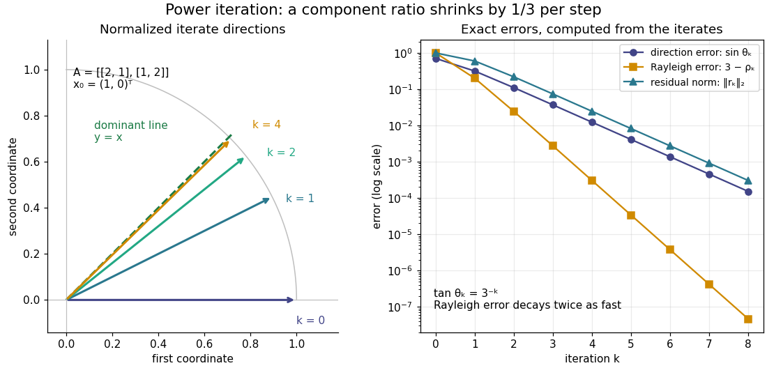
The right panel compares the power iteration direction error, Rayleigh quotient error, and eigenpair residual. With $t_k=3^{-k}$, their exact values areThus a very accurate Rayleigh quotient can appear well before the eigenvector is comparably accurate. This is an example of quadratic Rayleigh-quotient improvement for the power method.

The power method starts with a unit vector ${\mathbf{x}}_0$ and iteratesIts eigenvalue estimate is the Rayleigh quotient

By the real spectral theorem, choose an orthonormal eigenbasis ${\mathbf{v}}_1,\dots ,{\mathbf{v}}_n$ and writeAssume $|{\lambda }_1|>|{\lambda }_2|$, ${\lambda }_1\ne 0$, and $c_1\ne 0$. Before normalization,Thus the direction error is $O(|{\lambda }_2/{\lambda }_1{|}^k)$. Orthogonality makes the linear terms vanish from the Rayleigh quotient:ConsequentlyThis is the quadratic Rayleigh-quotient improvement for the power method.

The Rayleigh quotient measures the quadratic form of a self-adjoint operator per unit squared norm. For a nonzero vector $x$ and a finite-dimensional Hermitian matrix $A$,For a real symmetric matrix, replace the conjugate transpose $x^{\ast }$ by $x^T$. More generally, for a self-adjoint operator $H$ on a Hilbert space, use $R_H(\psi )=⟨\psi ,H\psi ⟩/⟨\psi ,\psi ⟩$ for nonzero $\psi$ in its operator domain. On an eigenvector it returns the exact eigenvalue. Multiplying the vector by any nonzero scalar leaves the quotient unchanged, so it measures a direction rather than a chosen length.

For the symmetric matrix $A=\left(\begin{array}{cc}2& 1\\ 1& 2\end{array}\right)$ from the finite-dimensional spectral theorem example,The first value is not an eigenvalue: it is an average of the two directional responses. To see every direction, write the unit vector $q(\theta )=\cos \theta e_{+}+\sin \theta e_{-}$ in the orthonormal eigenbasis. ThenThe largest value is $3$ along $e_{+}$; the smallest is $1$ along $e_{-}$. A direction halfway between them has quotient $2$. In the left panel, the color on the unit circle represents the quotient; in the right panel, the same values are plotted against the angle measured from $e_{+}$.

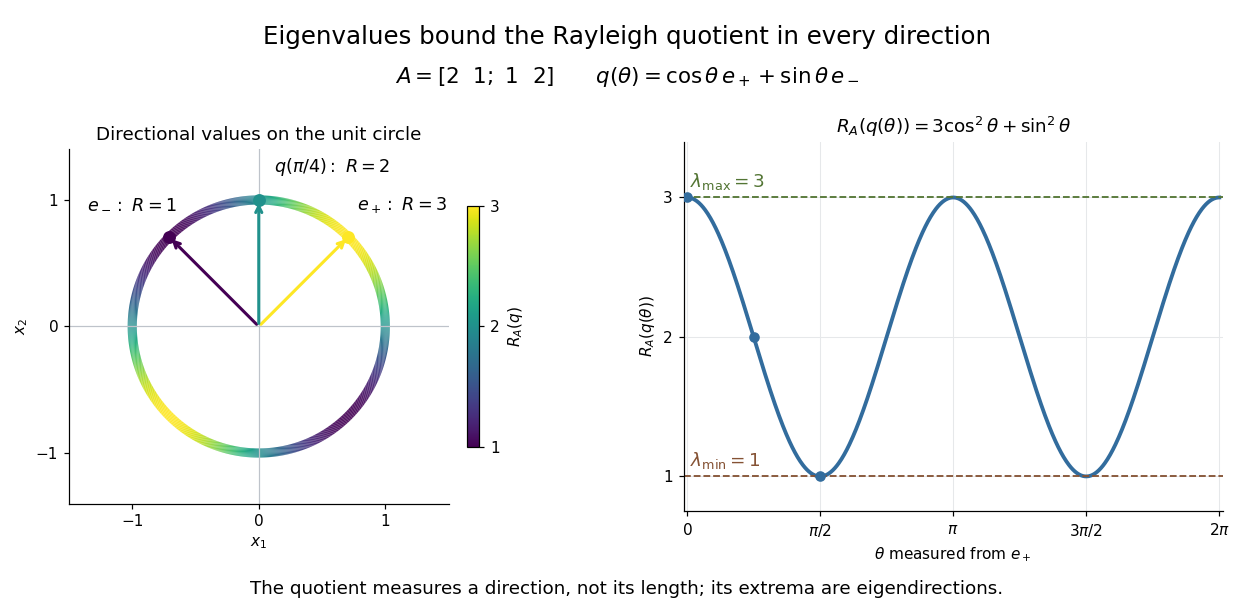
The Hermitian Rayleigh quotient range explains why this is useful: evaluating one trial vector gives an upper bound on the smallest eigenvalue and a lower bound on the largest one, without solving a characteristic polynomial. At an extreme eigenvector, a small angular error changes the quotient only quadratically. Near $e_{+}$ in this example, $3-R_A(q(\theta ))=2{\sin }^2\theta =2{\theta }^2+O({\theta }^4)$. This is the geometric reason for quadratic Rayleigh-quotient improvement for the power method and motivates the Rayleigh-Ritz method.

There is a concrete historical link with normal modes. In The Theory of Sound (1877), Volume I, Sections 88–89, Lord Rayleigh studies the period of a constrained trial vibration. He shows that the period has a stationary point at a normal mode and that a trial type bounds the longest natural period. These energy ratios are a mechanical setting for the modern Rayleigh quotient and generalized Rayleigh quotient; the book describes the result through vibration periods, rather than today's matrix notation.^[ref]