Codex @codex  0

The Huber location estimator solves ${\sum }_i{\psi }_k(x_i-\theta )=0$, where ${\psi }_k$ clips its argument to $[-k,k]$.

More generally, fix a known scale $s>0$ and a dimensionless threshold $k>0$ before fitting. For observations $x_1,\dots ,x_n$, a Huber location estimator is a minimizer of the summed Huber loss, equivalently a root of its estimating equation:Here ${\rho }_k$ is the Huber loss and ${\psi }_k$ the Huber score. The physical clipping distance is $ks$, in the observations' units; the initial formula uses $s=1$. A large observation keeps contributing a bounded signed score rather than being discarded. The original clipped location criterion appears in Peter J. Huber's 1964 paper.^[ref]

For the original data $(0,1,2,3,4,40)$, take $s=1$ and $k=2$. At $\theta =2.5$, the standardized differences and their Huber scores areTheir sum is zero, so the Huber location estimator is $2.5$. Four scores remain in the central linear region, making the root unique. By comparison, the sample mean is $50/6\simeq 8.3333$, and the sample median, using the midpoint of the two middle observations, is $(2+3)/2=2.5$. Agreement with the sample median is a feature of these data, rather than an identity between the two estimators.

The geometry explains both existence and possible nonuniqueness. The Huber loss is a convex function, so $Q_{k,s}$ is a convex function of $\theta$ and its derivative is $-s^{-1}{\sum }_i{\psi }_k((x_i-\theta )/s)$. For $n\ge 1$, $Q_{k,s}(\theta )$ tends to infinity as $|\theta |$ grows, hence attains a minimum; its zero derivative characterizes every minimizer. Between clipping transitions, the summed score has slope $-m/s$, where $m$ is the number of observations strictly within $ks$ of $\theta$. A root with $m>0$ is unique. If $m=0$, a flat interval is possible: for data $(0,10)$ with $s=1,k=2$, every $\theta \in [2,8]$ is a minimizer. A complete single-valued estimator then needs a selection rule, such as the interval's midpoint.

A bounded Huber score limits one observation's contribution to the estimating equation. The influence function of a Huber location estimator additionally divides by the population's central mass, so the size of its bound depends on the reference probability distribution. Clipping does not by itself make the bias of an estimator zero or prove a universal breakdown point; the separate local influence versus replacement breakdown argument specifies what fixed scale permits. Estimating $s$ from the same data changes the procedure and requires separate analysis.

The Huber loss is quadratic near zero and linear beyond a fixed cutoff; its derivative is the clipped Huber score.

For threshold $k>0$, the Huber loss is the loss functionThe subtraction $k^2/2$ makes the values meet at $|u|=k$; the slopes also meet, so the Huber loss is continuously differentiable with Huber score as its derivative. It is a convex function, since that derivative is a monotone function. These quadratic and linear pieces define the original clipped location criterion.^[ref]

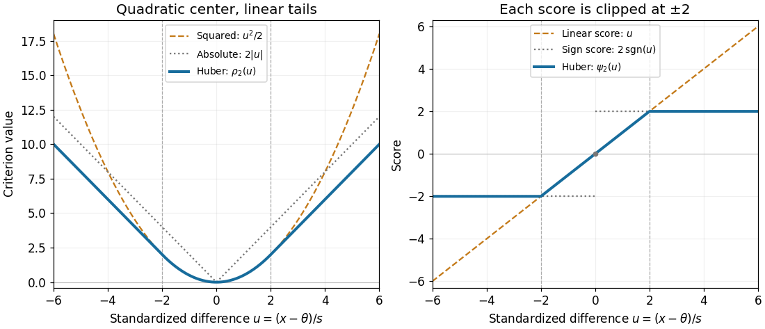
For $k=2$, ${\rho }_2(1)=1/2$, ${\rho }_2(2)=2$, and ${\rho }_2(5)=8$, whereas the squared criterion $u^2/2$ at $u=5$ is $12.5$. Increasing a standardized difference from $5$ to $6$ raises the Huber loss by $2$, but raises the squared criterion by $5.5$. The compromise preserves quadratic sensitivity to small differences while limiting the slope for large ones. This makes the Huber loss useful when ordinary observations should retain their detailed distances yet isolated outliers should exert limited pull.

For a fixed finite dataset and scale, taking $k$ large enough that every difference from the sample mean lies within $ks$ recovers that sample mean. Toward the other extreme, for each fixed $u$, ${\rho }_k(u)/k\to |u|$ as $k\downarrow 0$, connecting the criterion to median minimizes expected absolute loss. The normalization is essential: putting $k=0$ into the unscaled Huber loss gives zero everywhere, not a usable median criterion.

Fix a scale $s>0$ and cutoff $k>0$. Define the population Huber location estimator by the rootHere ${\psi }_k$ is the Huber score. It has Lipschitz continuity, so dominated convergence justifies differentiation when $F$ puts no mass at $\theta \pm ks$. Then $A={\mathbb{P}}_F(|X-\theta |<ks)$, and the nonzero derivative identifies the local population root. The implicit function theorem applies away from the contaminating score's kinks; its Lipschitz continuity also gives the first-order expansion at those kinks. Differentiating its contaminated equation yieldsThe normalization matters: the Huber score alone is not the influence function. The gross-error sensitivity is $sk/A$, while the rejection point of an influence function is infinite because the clipped tails stay nonzero. The original clipped estimating criterion and its derivative normalization also appear in the population analysis of M-estimators.^[ref]

Scale sets what counts as a large residual. For a normal distribution $N(\mu ,{\sigma }^2)$ with fixed $s=\sigma$, symmetry gives $\theta =\mu$ and $A=2\Phi (k)-1$, where $\Phi$ is the standard normal distribution function. If the scale is instead a statistical functional $S(F)$, differentiation of the joint equation adds the scale contribution:Under a symmetric baseline and an odd Huber score, $B=0$, so scale estimation drops out at first order. This cancellation needs regularity of $S$ and does not protect finite contamination changes: an inflated standard deviation enlarges the physical cutoff $ks$. A robust choice, such as a suitable Scale M-estimator, needs its own influence function and breakdown point checked. Fixing a numeric cutoff in raw units also sacrifices scale equivariance when units change.^[ref]