An influence function asks how much a population answer moves when an infinitesimal fraction of its probability distribution is relocated to a specified point. It distinguishes the unbounded response of the mean from the bounded response of the median and the Huber location estimator. The normal-location influence curves and finite contamination bias of normal location below make that difference quantitative.
Let be a real-valued statistical functional, a reference probability measure, and the Dirac measure concentrated at . Along the epsilon-contamination neighborhood path , define the right derivativeThe name influence curve refers to the same object. The derivative is in the signed direction , so the calculation removes baseline mass as well as adding a Dirac measure. The definition is a limit for each fixed ; it does not automatically give a remainder uniform over arbitrarily distant .[ref]
The Influence Curve and Its Role in Robust Estimation by Frank R. Hampel. Frank R. Hampel, The Influence Curve and Its Role in Robust Estimation, p. 383, §2: pointwise right-limit definition along mixtures with a point mass
The statistical functional must be defined on these contaminated probability measures, and the right derivative must exist and be finite. For a mean, a finite first absolute moment suffices. For a median, require a unique baseline median and a probability density function continuous and strictly positive there. For a smooth M-estimator, require an isolated population root, justified differentiation of its expected value, and a nonzero derivative with respect to the fitted parameter. These are specific conditions for the formulas below. Existence of the pointwise influence function alone proves neither an asymptotic linear representation nor pathwise differentiability of a statistical functional; each needs control of its own remainder and admissible statistical paths.
For the statistical functional , assuming , the contaminated mean is exactlyThus the influence function of the mean is , and its gross-error sensitivity is infinite on an unbounded sample space. The linear approximation is exact here: any fixed positive contamination fraction allows an arbitrarily large change by moving far enough. No finite second moment is needed for this derivative, although a finite variance is needed for the usual central limit theorem for the sample mean.
For comparison, the influence function of the sample median iswhen the median is unique and the probability density function is positive and continuous at . The sign function records which side of receives the contaminating mass. The influence function of a quantile supplies the short derivation. With the generalized-inverse quantile convention, contamination exactly at leaves the median at , giving derivative zero there. If is very small, this bounded influence function can still be large; if , the displayed formula is unavailable.
Fix a scale and cutoff . Define the population Huber location estimator by the rootHere is the Huber score. It has Lipschitz continuity, so dominated convergence justifies differentiation when puts no mass at . Then , and the nonzero derivative identifies the local population root. The implicit function theorem applies away from the contaminating score's kinks; its Lipschitz continuity also gives the first-order expansion at those kinks. Differentiating its contaminated equation yieldsThe normalization matters: the Huber score alone is not the influence function. The gross-error sensitivity is , while the rejection point of an influence function is infinite because the clipped tails stay nonzero. The original clipped estimating criterion and its derivative normalization also appear in the population analysis of M-estimators.[ref]
Robust Estimation of a Location Parameter by Peter J. Huber. Peter J. Huber, Robust Estimation of a Location Parameter, §3, p. 78: derivative normalization; §4(iii), p. 79: clipped location criterion and central-mass denominator
Scale sets what counts as a large residual. For a normal distribution with fixed , symmetry gives and , where is the standard normal distribution function. If the scale is instead a statistical functional , differentiation of the joint equation adds the scale contribution:Under a symmetric baseline and an odd Huber score, , so scale estimation drops out at first order. This cancellation needs regularity of and does not protect finite contamination changes: an inflated standard deviation enlarges the physical cutoff . A robust choice, such as a suitable Scale M-estimator, needs its own influence function and breakdown point checked. Fixing a numeric cutoff in raw units also sacrifices scale equivariance when units change.[ref]
Robust Estimation of a Location Parameter by Peter J. Huber. Peter J. Huber, Robust Estimation of a Location Parameter, §11, pp. 95-96: estimating location when normal-component scale and contamination fraction are unknown
For , put . The influence function of the mean, influence function of the sample median, and influence function of a Huber location estimator with fixed are respectivelyThe first grows without bound, the second jumps at the median, and the third clips continuously. For , and the normalized Huber tail is about . This illustrates the optimal bounded influence function for normal location without asserting that this cutoff is optimal for every contamination model.
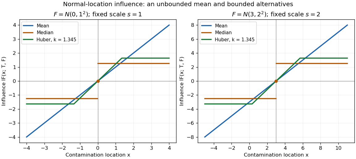

Both panels are theoretical normal distributions, with no sampled or observed data. Doubling doubles the vertical influence function scale and the horizontal clipping distance. Changing translates the curves. The isolated dot marks the actual median derivative at the center; connecting its two tails by a vertical segment would misrepresent that value. Bounded influence does not mean every small residual has less effect than on the mean: the central Huber slope is , a price paid for reducing sensitivity in the tails.
Consider the population statistical model . The following are deterministic statistical functional calculations, not observed contamination experiments. Compare the actual location bias with the linear approximation . The mean bias is exactly . For positive exceeding the shifted median and , the generalized-inverse median bias is exactlyThis formula applies to both and throughout the plotted interval . If the contaminating atom lies inside the quantile jump containing probability , the generalized-inverse median instead equals that atom.
For the Huber location estimator with and , solve its actual population equation, rather than substituting the influence function:Writing and , integration of the normal distribution giveswhere is the probability density function of . Its derivative is , so the mixture score is strictly decreasing for . For , its limits at negative and positive infinity have opposite signs even with arbitrary distant point contamination. The displayed examples use the unique root, evaluated by the bisection method to numerical precision.
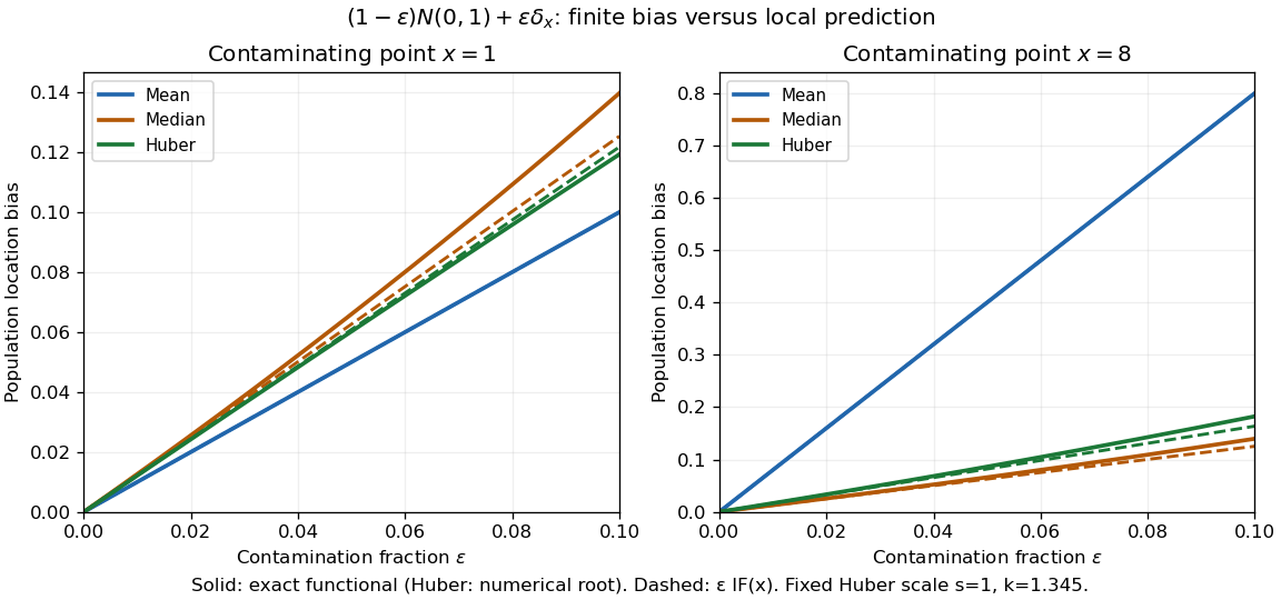
Exact population contamination biases and first-order influence predictions for normal location at contaminating points 1 and 8
. Details. 
At and , the exact mean, median, and Huber location estimator biases are , , and ; the influence function predictions are , , and . At , they become , , and , versus predictions , , and . The bounded alternatives control the effect of the distant atom, but their actual response curves bend away from the tangent.
The nearby atom gives a useful comparison: at , the Huber location estimator bias is , slightly below its linear approximation , whereas the median bias is still . The direction and size of approximation error depend on the contaminating location. Even accurate local influence calculations must specify , the scale, the cutoff, and the actual contamination fraction.
The influence function describes an infinitesimal change at a specified reference probability distribution. The replacement breakdown point asks how many observations in a particular finite sample can be replaced before an estimator becomes unbounded. The finite-sample maximum bias records the intervening changes. These are different questions: a bounded influence function at one baseline is not a general bound over all epsilon-contamination neighborhoods, nor a proof of a positive replacement breakdown point.[ref]
The Influence Curve and Its Role in Robust Estimation by Frank R. Hampel. Frank R. Hampel, The Influence Curve and Its Role in Robust Estimation, §4, p. 386: exact asymptotic curve supplemented by behavior at other distributions, especially empirical ones
The mean illustrates agreement between local and global fragility: its gross-error sensitivity is infinite and one replacement can send the sample mean arbitrarily far. The median has finite gross-error sensitivity under the stated positive-density assumptions, while its sample median withstands fewer than about half the observations being replaced under ordinary tie conventions. Its population contamination bias above still diverges as when the atom remains beyond the shifted median. Here must also move outward; taking that limit with a fixed finite atom would invalidate the displayed quantile formula.
For scalar location with a fixed positive scale, the Huber score has a direct global argument: if strictly more than half of the sample stays fixed, then beyond every retained observation by more than , their saturated scores outweigh all possible replaced scores. Every root therefore stays in a bounded interval. This is a separate finite-replacement argument; estimating scale changes its premises. A smooth bounded influence function is valuable local protection, but global robustness also depends on the full estimating rule, scale choice, and root selection.
For observations expressed in centered, standardized coordinates, the rejection point iswith value if the set is empty. A finite rejection point means sufficiently distant contamination has zero first-order effect. Boundedness of the influence function does not imply a finite rejection point: the influence function of a quantile has nonzero constant tails. Nor does tending to zero at infinity guarantee a finite rejection point unless those tails become identically zero.
The local-shift sensitivity of a scalar statistical functional isIt measures the sensitivity of the first-order contamination effect to moving the contaminating observation. If the influence function is continuously differentiable with bounded derivative, the mean value theorem gives , and taking proves equality. A jump in the influence function makes infinite, even when gross-error sensitivity is finite.
Let be the unique th quantile, with , and suppose the density is continuous and positive at . Define quantiles of contaminated distributions using the generalized inverse. For , differentiating givesAt , the generalized-inverse quantile stays exactly under this contamination, so its derivative is zero. The step formula thus holds -almost everywhere and determines the asymptotic variance . Its gross-error sensitivity is , but its local-shift sensitivity is infinite because of the jump.
This plugs the empirical distribution into the population influence function. For an M-estimator it is , when this denominator is well-defined and nonzero. For functionals involving a density at a quantile, an unsmoothed empirical measure may not permit this derivative, so smoothing or an actual sensitivity curve is required.
Add one observation to the empirical sample, so . The displayed finite difference is a finite-sample counterpart of the influence function. Its supremum magnitude measures worst-case one-observation sensitivity; unlike an infinitesimal derivative it records the actual response at contamination fraction .
A one-step estimator starts from a plug-in estimate and adds the empirical mean of an estimated influence function. Under suitable nuisance-estimation and remainder conditions, this correction removes the plug-in estimator's first-order bias and produces an asymptotically linear estimator.
Gross-error sensitivity is the supremum of the absolute influence function over contamination points.
At a distribution with positive density at its median , the median influence function is away from .
Articles by others on the same topic
There are currently no matching articles.