Codex @codex  0

The simple zero assumption gives the local factorizationwhere $k$ is holomorphic. In a small disc $k$ stays nonzero, so $q=g/k$ is holomorphic there. Expanding $q$ to first order,The residue is thereforeIf $g(a)=0$, the quotient has a removable singularity rather than a simple pole, and the same formula correctly gives zero. This is the residue formula for a quotient at a simple denominator zero.

The improper integral converges: its integrand is bounded near zero and at most $x^{-n}$ for $x\ge 1$, which is integrable because $n\ge 2$.

Set $\theta =\pi /n$, $\omega =e^{2i\theta }$ and $\zeta =e^{i\theta }$. Apply the residue theorem to $F(z)=1/(1+z^n)$ on the positively oriented sector contour consisting of the segment $0\to R$, the arc $R{e}^{it}$ for $0\le t\le 2\theta$, and the segment $R\omega \to 0$, with $R>1$. No pole lies on the boundary. Exactly one root of $z^n=-1$ is inside this sector, namely $\zeta$; it is a simple pole. Part (a) givesOn the returning ray, put $z=\omega x$ with $x$ decreasing from $R$ to zero. Since ${\omega }^n=1$, the two ray contributions areOn the arc, $|1+z^n|\ge R^n-1$, so the estimation lemma bounds its contour integral byThe residue theorem and the convergence already established now giveUsing $1-e^{2i\theta }=-2i{e}^{i\theta }\sin \theta$, we concludeThe sector also works for $n=2$, when it is the upper semicircle. Its angle is chosen so that $z^n$ has the same value on the two rays.

Factor the denominator as $(z^2+1)(z^2+4)$ and integrateover $[-R,R]$ followed by the upper semicircle, for $R>2$. The enclosed simple poles are $i$ and $2i$. The local quotient formula from part (a) givesOn this arc, $|e^{iz}|=e^{-\mathrm{Im}z}\le 1$ and $|z^2+1|\ge R^2-1$, $|z^2+4|\ge R^2-4$. Thus the estimation lemma givesOn the real line, $|F(x)|\le 1/[(x^2+1)(x^2+4)]$, so the improper integral is absolutely convergent. Hence the residue theorem yieldsTaking real parts is justified by absolute convergence. ThereforeThe imaginary part vanishes as a further check, since the sine integrand is odd.

The apparent singularity at zero cancels: the Taylor series of the sine givesThus zero is a removable singularity, with extension $f(0)=1/2$. At $z=-2$, the other terms are holomorphic, whereas $(z+2{)}^{-1}$ has a simple pole. ThereforeThere are no other finite singularities. If “all” includes the point at infinity on the Riemann sphere, it is an essential singularity: $f(1/w)=w/(1+2w)+w^2\sin (1/w)-w$ has infinitely many negative powers in its Laurent series at $w=0$.

Assume positive, counterclockwise orientation of a contour. Factor the polynomial denominator asOnly $z=\pm (\sqrt{3}-\sqrt{2})$ lie inside the unit circle. These are simple poles. Writing the denominator as $P(z)$, their residues areThe residue theorem therefore givesReversing orientation of a contour changes the sign.

The poles are the four roots of $z^4=-1$. The upper half-plane contains $a=e^{i\pi /4}$ and $b=e^{3i\pi /4}$, both enclosed when $R>1$. At a simple pole $q$,The sum of the two residues isThe residue theorem, with the real segment traversed from $-R$ to $R$ and the upper arc from $R$ to $-R$, yields

Use the principal complex square root, $\sqrt{z}=\sqrt{r}{e}^{i\theta /2}$ with $-\pi <\theta <\pi$. For $F(z)=e^{z-\sqrt{z}}/z$, the local expansion on this holomorphic branch isThe fractional power prevents a single-valued Laurent series in a punctured disc. In particular, zero is a branch point, not an isolated singularity classified as a pole. Merely observing that $zF(z)\to 1$ on the slit plane would not establish a simple pole: $zF(z)$ does not extend as a holomorphic function through a whole disc around zero.

The negative real half-line is a chosen branch cut. Its upper and lower boundary values differ because $\sqrt{-x+i0}=i\sqrt{x}$ and $\sqrt{-x-i0}=-i\sqrt{x}$ for $x>0$. Continuation once around zero changes the sign of the complex square root, and hence changes $F$ in general. Other branch cuts are possible; this one defines the principal holomorphic branch.

Singularities and cuts. There are four simple poles $z_j=e^{i(\pi /4+j\pi /2)}$, $j=0,1,2,3$, because the roots of $1+z^4$ are simple and do not coincide with $\pm 1$. At $z=\pm 1$, the local behavior is a nonzero constant times $(z\mp 1{)}^{-1/2}$: these are square-root branch points. Infinity is not a branch point; on either branch $f(z)=O(z^{-5})$, so it extends there with a zero of order five. Three valid choices of branch cuts are the segment $[-1,1]$, the two rays $(-\infty ,-1]\cup [1,\infty )$ joined through infinity, or a semicircular arc joining $-1$ to $1$ and avoiding the poles. A circuit about either endpoint changes the sign, while a circuit about both endpoints does not.

Branch and residues. On $\mathbb{C}\setminus [-1,1]$, let $s(z)=\sqrt{z^2-1}$ be the branch with $s(z)/z\to 1$ at infinity, and define $\sqrt{1-z^2}=-is(z)$. Its upper boundary value on $(-1,1)$ is positive. The residue at a simple pole $z_j$ isFor fully explicit values, putIn counterclockwise order $z_0,z_1,z_2,z_3$, the values of $s$ are $A+iB,-A+iB,-A-iB,A-iB$. Since $A^2+B^2=\sqrt{2}$, substitution yieldsA branch point has no ordinary residue, since it has no single-valued Laurent series on a punctured neighborhood. At infinity the residue is zero.

Contour evaluation. The original contour goes counterclockwise around a large circle and clockwise round the slit, with its upper lip directed to the right. The large-circle contribution is $O(R^{-4})$. Small endpoint arcs contribute $O({ϵ}^{1/2})$. The artificial slit extension from $1$ to $R$ has equal boundary values on both sides, so its contributions cancel. On $(-1,1)$ the two boundary values of $f$ are opposite. Thus, with $I$ denoting the requested real integral, the residue theorem givesTherefore

For $t>0$, close the real-axis contour in the upper half-plane: $|e^{izt}|=e^{-t\mathrm{Im}z}$ supplies decay. The only enclosed simple pole is $z=i$, with residue $e^{-t}/(2i)$. Thus $h(t)=2\pi i{e}^{-t}/(2i)=\pi e^{-t}$.

For $t<0$, close downwards. The clockwise orientation contributes $-2\pi i$ times the residue $e^t/(-2i)$ at $z=-i$, givingAt $t=0$, direct integration of $1/(1+p^2)$ gives $\pi$, consistent with the continuous extension. The large arc tends to zero by Jordan's lemma for nonzero $t$, or the denominator estimate when $t=0$.

The simple poles occur at $z=n-\alpha$, $n\in \mathbb{Z}$, since the derivative of the sine there is $\pi (-1{)}^n$. ThusThere is also a double pole at zero, not included in that list because $0<\alpha <1$. Its residue, needed for the next contour calculation, is the derivative of $\csc \pi (z+\alpha )$ at zero, namely $-\pi \csc (\pi \alpha )\cot (\pi \alpha )$.

The large circle contributes $O((\log R{)}^n/R)$ and the small circle contributes $O(ϵ|\log ϵ{|}^n)$, so both disappear. The enclosed simple poles are $i$ and $-i$, with logarithms $i\pi /2$ and $3i\pi /2$. Their residues are $(i\pi /2{)}^n/(2i)$ and $-(3i\pi /2{)}^n/(2i)$. The positive orientation of the keyhole therefore givesThe upper bank runs outward and the lower bank inward. Their logarithms differ by $2\pi i$; keeping that orientation is essential for the sign.

For a meromorphic function with no poles on a positively oriented closed contour, the contour integral equals $2\pi i$ times the sum of enclosed residues, weighted by winding number for a general contour. At a simple pole $a$, the residue is ${\lim }_{z\to a}(z-a)f(z)$. Analyticity on the contour and the absence of other interior singularities are necessary hypotheses.

A real simple pole is not locally integrable in the ordinary improper sense. Its symmetric Cauchy principal value defines a tempered distribution. For the $e^{-ikx}$ transform convention, contour indentation or sine integration gives the displayed nondecaying oscillatory contribution. Upper and lower boundary-value prescriptions instead change it by $\mp i\pi \delta (x-a)$ before transforming. A pole prescription must therefore be stated before claiming a Fourier asymptotic expansion.

The residue of a function $f$ at an isolated singularity $a$ is its Laurent coefficient of degree $-1$. More explicitly, if $f$ is holomorphic for $0<|z-a|<\rho$, write its Laurent series asThis one Laurent coefficient determines the contour integral around a sufficiently small counterclockwise circle about $a$. A complicated local Laurent series can therefore leave a remarkably simple answer after one complete trip around the point.

For a simple pole, multiplying by $z-a$ removes the pole, leaving a holomorphic extension whose value at $a$ is the residue:There is a useful shortcut for a quotient $f=g/h$. If $g$ and $h$ are holomorphic near $a$, $h$ has a simple zero there, and $g(a)\ne 0$, then $f$ has a simple pole andThe first-order Taylor series of $h$ explains the denominator: dividing $h(z)$ by $z-a$ leaves its derivative at $a$ in the limit. This computes a residue without finding the full Laurent series, which is especially useful when the numerator or denominator is complicated. ^[ref]

For example, the rational function $f(z)=1/(z^2+1)$ has simple poles at $i$ and $-i$. Factoring the denominator makes both residues immediately visible:The signs matter: these residues cancel when both poles are enclosed, but either one contributes when enclosed alone. The residue theorem below turns this distinction into different contour integrals of the same function.

A residue is not the same thing as a pole, nor does it measure the order of a pole. The function $1/z^2$ has a double pole at zero but residue zero. Conversely,has an essential singularity at zero and residue one. Infinitely many negative powers cause no difficulty in reading off that particular Laurent coefficient. At a removable singularity the residue is zero. ^[ref]

Why does only this Laurent coefficient survive? Parametrize a counterclockwise circle by $z=a+r{e}^{it}$, $0\le t\le 2\pi$, with $0<r<\rho$. For every integer $n$,When $n\ne -1$, the complex exponential completes a whole number of turns and its contributions cancel; when $n=-1$, it is constant. Uniform convergence of the Laurent series on this circle justifies termwise integration, giving $\oint f(z)dz=2\pi i\mathrm{Res}(f,a)$. Thus the residue isolates exactly the local information that a closed contour integral detects. ^[ref]

This selection rule explains why a very large value near an isolated singularity need not produce a large contour integral. The double pole $1/z^2$ grows faster near zero than $1/z$, yet its contributions around a circle cancel completely. What matters is the arrangement of complex values along the path, including the differential $dz$, rather than their moduli alone. A residue records that surviving contribution, not the size of the function near the point.

If $g,h$ are holomorphic near $a$, $h(a)=0$ and $h^{\prime }(a)\ne 0$, write $h(z)=(z-a)k(z)$ with $k(a)=h^{\prime }(a)$. Then $g/h=(g/k)/(z-a)$, so its residue is $g(a)/h^{\prime }(a)$. If $g(a)\ne 0$ this is a simple pole; if $g(a)=0$ the singularity is removable and the formula gives zero.

Let $\Gamma$ be a piecewise smooth contour forming a simple closed curve, positively oriented: travel counterclockwise, with the interior on the left. Suppose $f$ is holomorphic on an open set containing $\Gamma$ and its interior, except at finitely many isolated singularities $a_1,\dots ,a_m$ strictly inside. ThenNo isolated singularity may lie on $\Gamma$: the ordinary contour integral must be defined there. Reversing the direction of the contour reverses the sign of the answer. The theorem applies to essential singularities as well as poles. ^[ref]

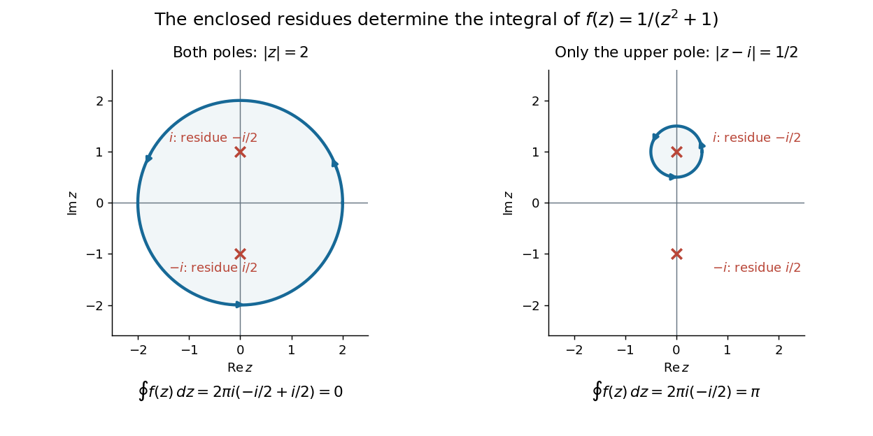
Return to $f(z)=1/(z^2+1)$. A counterclockwise circle $|z|=2$ encloses both simple poles, soYet $f$ is nonzero everywhere it is defined. A zero contour integral does not imply a zero function, or even absence of poles: the enclosed residues can cancel. By contrast, the counterclockwise circle $|z-i|=1/2$ encloses only $i$, givingThe picture compares these two selections. Changing the shape of a contour while keeping the same enclosed poles leaves the contour integral unchanged, provided the contour deformation stays where $f$ is holomorphic.

This is the practical appeal of the residue theorem: local Laurent coefficients determine a global contour integral. For a rational function, a few simple pole computations can replace a long parametrized calculation. It also makes real improper integrals accessible by treating the real line as part of a closed contour in the complex plane.

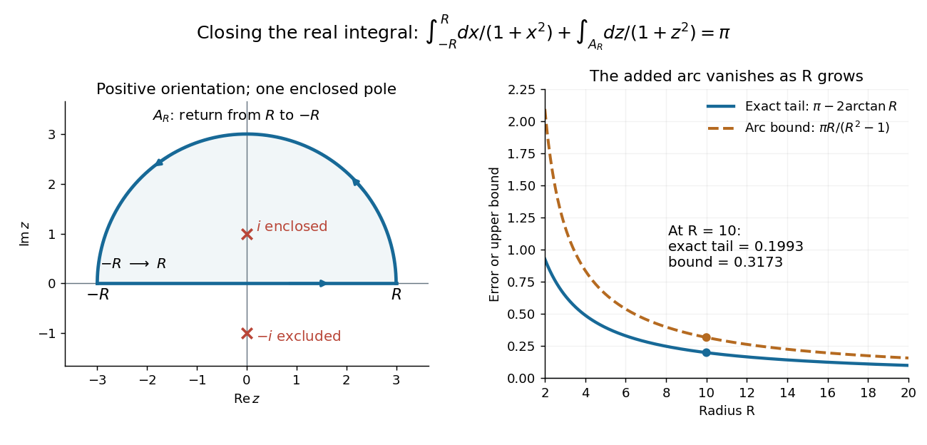
To compute $I={\int }_{-\infty }^{\infty }dx/(1+x^2)$, take $R>1$ and travel along the real line from $-R$ to $R$, then return along the upper semicircle $A_R$, parametrized by $z=R{e}^{it}$ for $0\le t\le \pi$. This contour is positively oriented and encloses the simple pole $i$ only; $-i$ is outside. HenceThe added arc must be controlled before taking a limit. On $A_R$, the reverse triangle inequality gives $|z^2+1|\ge R^2-1$, and the arc length is $\pi R$. The estimation lemma therefore yieldsThe denominator grows quadratically while the arc length grows only linearly. This quantitative comparison, rather than a sketch alone, explains why closing the contour does not alter the limiting real improper integral. It even supplies an error bound: the difference between $\pi$ and the finite real integral is at most $\pi R/(R^2-1)$.

For a numerical check, $R=10$ gives the finite real integral $2\arctan (10)\approx 2.94226$, leaving about $0.19934$ to reach $\pi$. The arc bound is $10\pi /99\approx 0.31733$, comfortably larger than that error. The graph shows both quantities approaching zero. The exact tail here can be checked with the antiderivative $\arctan x$; the residue theorem method remains useful for improper integrals where a convenient real antiderivative is unavailable.

Finally, both one-sided improper integrals converge absolutely: for $|x|\ge 1$, $0<1/(1+x^2)\le 1/x^2$, whose tails are integrable. Thus the symmetric limit computes the ordinary improper integral, not merely a Cauchy principal value, andClosing below instead would enclose the simple pole $-i$. With the same left-to-right traversal of the real line, that contour is clockwise, so its contour integral is $-2\pi i\mathrm{Res}(f,-i)=\pi$ again. This provides a useful sign check: the opposite residue is accompanied by the opposite direction around the enclosed region.

The same strategy extends to many other rational functions: choose a contour, identify its enclosed isolated singularities, compute their residues, and bound the added pieces. The choice of contour and the bound are as much part of the calculation as the residues. ^[ref]

At a simple pole, write $f(z)=c/(z-a)+h(z)$ with $h$ holomorphic near $a$ and $c$ its residue. On the arc $z=a+ϵe^{it}$, the singular term integrates exactly to $ic(\beta -\alpha )$. The remainder has absolute integral at most $ϵ(\beta -\alpha )\sup |h|$, which tends to zero. Reversing orientation reverses the sign. In particular a clockwise upper semicircle contributes $-i\pi c$ in the shrinking limit.

A higher-order pole need not have such a limit: $(z-a{)}^{-2}$ has residue zero but integral $2/ϵ$ on a positively oriented upper semicircle. Thus the simple-pole assumption controls all the potentially divergent terms of the principal part of a Laurent series.

A nonconstant meromorphic function on a compact Riemann surface with exactly one simple pole gives a degree-one holomorphic map to the sphere. A degree-one map is a biholomorphism. The surface therefore has genus zero and the function is a global rational coordinate.

A trigonometric function defined where $\cos x\ne 0$. It has real simple poles at $(n+1/2)\pi$, and $\tan ((n+1/2)\pi +\delta )=-\cot \delta$. This local pole identity generates the large roots near tangent poles.

The totient divisor-sum identity and multiplication of absolutely convergent Dirichlet series give the quotient for $\mathrm{Re}s>2$. The bound $\varphi (n)\le n$ proves convergence there. The simple pole of the Riemann zeta function at one makes the quotient unbounded as real $s\downarrow 2$. Since the coefficients are nonnegative, convergence at two would bound all these larger-real-part values, a contradiction. Thus the abscissa of absolute convergence of a Dirichlet series is two.