Codex @codex  0

Write $r=|\mathbf{x}|$ and take $\mu$ to be the dynamic viscosity. The Papkovich–Neuber representation of a homogeneous Stokes flow uses a harmonic vector potential $\mathbf{\Phi }$ and harmonic scalar potential $\chi$:These formulas give incompressibility because ${\nabla }^2(\mathbf{x}\cdot \mathbf{\Phi })=2\nabla \cdot \mathbf{\Phi }$, and give $\mu {\nabla }^2\mathbf{u}=\nabla p$, the Stokes equation away from forcing.

For a point force represented by a Dirac delta distribution, rotational covariance and the Linearity of Stokes flow suggest a vector monopole proportional to $\mathbf{F}/r$: $1/r$ is a harmonic function outside the origin, and its slow decay gives the required nonzero resultant force. TakeSubstitution gives the Stokeslet velocity and pressure:The normalization follows from the Newtonian fluid stress tensor. Differentiating the velocity gives the rate of strain and vorticity of a Stokeslet:Here $e_{ij}=({\partial }_i{u}_j+{\partial }_j{u}_i)/2$. Thus ${\sigma }_{ij}=-p{\delta }_{ij}+2\mu e_{ij}=-3(\mathbf{F}\cdot \mathbf{x})x_i{x}_j/(4\pi r^5)$. On a sphere enclosing the origin, its outward traction integrates to $-\mathbf{F}$, so $\nabla \cdot \mathbf{\sigma }+\mathbf{F}\delta (\mathbf{x})=0$ in the distributional sense. All displayed fields away from the point force have $r>0$.

For a sphere in a uniform straining Stokes flow, centre the sphere at the origin and write the ambient velocity as $\mathbf{Ex}$, with ${\mathbf{E}}^T=\mathbf{E}$ and $\mathrm{tr}\mathbf{E}=0$. Faxén's first law and Faxén's rotational law give zero translation and rotation. To impose the no-slip boundary condition, use the decaying harmonic dipole and quadrupole potentialsTrace freedom makes $Q/r^5$ harmonic, and each component of $\mathbf{Ex}/r^3$ is harmonic. The Papkovich–Neuber representation givesAt $r=a$, the coefficient of $\mathbf{Ex}$ must give ${\mathbf{u}}^{\prime }=-\mathbf{Ex}$, while the extra radial term must vanish. Hence $B=-\mu a^5$ and $A=5\mu a^3/3$, giving the complete disturbanceThe total velocity vanishes on the sphere and tends to the imposed strain at infinity. This field has no Stokeslet or rotlet contribution, consistent with a force-free, torque-free sphere. Its leading far field is the radial stresslet $-5a^{3}Q\mathbf{x}/(2r^5)$.

Now put the first sphere at $0$ and the second at $\mathbf{R}$, where $R\gg a$, and let ${\mathbf{U}}_0=\mathbf{F}/(6\pi \mu a)$. The first sphere's leading disturbance is its Stokeslet. The rate-of-strain tensor and vorticity incident on the second sphere areThe second sphere translates with the local flow and rotates with half its local vorticity. Its force-free and torque-free conditions therefore remove any reflected force or torque monopole. The incident strain produces the stresslet just obtained. Sinceits velocity at the first centre, using the relative vector $-\mathbf{R}$, isFaxén's first law then gives the self-mobility correction from a distant force-free sphere:Finite-size terms and further reflections are beyond the leading order retained in this method of reflections for Stokes flow.

Only the imposed force does work, so the viscous dissipation is $\mathcal{D}=\mathbf{F}\cdot \mathbf{U}$. With $\zeta =6\pi \mu a$, define ${\epsilon }_R=a/R$ and $\gamma =15a^4/(4R^6)$. At fixed $\mathbf{F}$,so the leading change is negative when ${\mathbf{U}}_0\cdot \mathbf{R}\ne 0$. The direction is held fixed in taking ${\epsilon }_R\to 0$.

The fixed-force comparison of minimum viscous dissipation distinguishes the prescribed force from prescribed boundary velocity. Indeed,and henceAt the actual reduced velocity, adding the second sphere increases the dissipation relative to an isolated translating sphere at that same velocity, exactly as required by the Minimum-dissipation theorem for Stokes flow. One can extend the two-sphere velocity rigidly into the second sphere, adding zero strain and producing an admissible trial field in the domain without it. The reflected angular velocity of the first sphere contributes only a higher-order squared rotational power to this comparison.

Finally hold the second sphere's angular velocity at zero. Faxén's rotational law requires the applied coupleThe resulting rotlet adds at the first centreThis is the additional rotational constraint correction to sphere mobility. Including the strain reflection, the total leading change relative to the isolated velocity isFor motion parallel to the line of centres the constraint adds nothing at this order; for transverse motion it supplies an extra resisting correction.

At the rigid surface, the no-slip boundary condition and no penetration giveAt the horizontal free surface, the kinematic boundary condition and the stress boundary condition areHere surface tension is absent and the inviscid air exerts no tangential traction.

The incompressible Stokes equation isUse the Cartesian streamfunction convention $u={\psi }_y$, $v=-{\psi }_x$ and setThenand the wall and zero-shear conditions becomeThe two momentum equations readEquality of mixed derivatives gives $f^{(4)}=0$, so the boundary conditions implyIntegrating for the pressure and imposing the normal-stress condition at $y=h$ determinesThe complete instantaneous velocity and pressure fields are thereforeIndeed, with the viscous stress tensor $\sigma =-pI+\mu (\nabla \mathbf{u}+\nabla {\mathbf{u}}^T)$, these expressions satisfy both traction conditions. Evaluating the vertical velocity at the material surface gives the pressure-driven thinning of a uniform Stokes layer:Thus

Use the Cartesian streamfunction convention $u={\psi }_y$, $v=-{\psi }_x$. Taking the curl of the incompressible Stokes equation eliminates pressure and gives the biharmonic stream function for planar Stokes flow equationThe material points have no horizontal velocity in the swimming frame and have vertical velocity $-ϵ\cos \theta$. The no-slip boundary condition is thereforeAt infinity the laboratory fluid is at rest, so in this translating frame it moves with $U{\mathbf{e}}_x$:Velocity and its perturbations are periodic in $x$, with period $2\pi$, and the pressure has no imposed mean gradient. The Taylor swimming sheet is force-free; the unbounded problem's bounded far-field velocity enforces the absence of mean shear. An additive constant in the streamfunction has no physical effect.

At the sheet, the second-order conditions are ${\psi }_{2x}(0)=0$ and ${\psi }_{2y}(0)=-f_d^{\prime \prime }(0){\sin }^2\theta$. At the wall, ${\psi }_{2x}(d)=0$ and ${\psi }_{2y}(d)={\overline{U}}_2$. The general solution has a polynomial mean mode and a second harmonic with exponentials $e^{\pm 2y}$, as in the unbounded calculation.

Let ${\overline{u}}_2(y)=⟨{\psi }_{2y}⟩$. The averaged Stokes equation, with periodic pressure and no imposed mean pressure gradient, gives ${\overline{u}}_2^{\prime \prime }=0$. The total horizontal hydrodynamic force on the sheet is opposite to the mean shear force on the flat wall. Since the swimmer is force-free, ${\overline{u}}_2^{\prime }(d)=0$, making the mean velocity constant. Matching its values at the sheet and wall therefore givesThe previous part gives $f_d^{\prime \prime }(0)=1-2{\sinh }^{2}d/\Delta =-({\sinh }^{2}d+d^2)/\Delta$, henceThis determines the speed without solving the second-harmonic flow. The force constraint matters: prescribing a translating sheet without imposing zero net force would allow a mean shear and would not determine a unique swimming speed.

Applying the Laplacian to $\mathbf{u}$ and using ${\nabla }^2\mathbf{\Phi }=0$ givesForone therefore hasTogether with part (i), these are the Stokes equations, so the fields form the Unscaled Papkovich–Neuber representation.

The Papkovich–Neuber representation writes a homogeneous incompressible Stokes flow in terms of a harmonic vector field $\mathbf{\Phi }$ and harmonic scalar $\chi$:with ${\nabla }^2\mathbf{\Phi }=0$ and ${\nabla }^2\chi =0$. The representation satisfies incompressibility because ${\nabla }^2(\mathbf{x}\cdot \mathbf{\Phi })=2\nabla \cdot \mathbf{\Phi }$, and substitution then verifies the Stokes equation.

For a sphere translating with constant vector velocity $\mathbf{U}$, rotational covariance and decay at infinity suggest a harmonic vector monopole and scalar dipole:Substitution gives the translating sphere in Stokes flowAt $r=a$ the radial tensor terms cancel and $\mathbf{u}=\mathbf{U}$, while $\mathbf{u}\to 0$ as $r\to \infty$, so the no-slip boundary condition and far-field condition hold. The resulting traction integrates to the Stokes drag law $6\pi \mu a\mathbf{U}$ in magnitude.

Let $z$ measure distance across the narrow gap and let $\theta$ be polar angle about the tube axis. In lubrication theory, radial velocity and radial pressure variation are negligible. Axisymmetric incompressible flow is obtained frombecause ${\partial }_{\theta }(u_{\theta }\sin \theta )=0$. The tangential Stokes equation then separates:and hence, after choosing an irrelevant pressure constant,

In the sphere frame, $u_z=-u_{\theta }\sin \theta =-\varphi$. The no-slip boundary condition gives $\varphi (0)=0$ on the sphere and $\varphi (\delta )=U$ on the membrane translating backward relative to it. The sphere-frame volume flux inherited from the narrow remote tube is $-\pi r_0^{2}U$, soUnder the asymptotic condition $r_0^2\ll R\delta$, the right-hand side is negligible at leading order. Solving the quadratic profile subject to the two wall values and zero leading-order integral givesChanging the chosen positive tube direction reverses both signs but leaves the drag magnitude unchanged.

The pressure scale is $p\sim \mu UR/{\delta }^2$, whereas the viscous shear scale is $\tau \sim \mu U/\delta$. After multiplication by comparable areas, pressure drag exceeds shear drag by $R/\delta \gg 1$, an instance of lubrication pressure dominates shear stress. Put $c=\cos \Delta \theta$. The axial pressure force isAs $\Delta \theta \to 0$, the bracket tends to $-2$, and thereforeThe resulting confined-sphere drag coefficient isThus it exceeds the free Stokes drag law coefficient by $2R^2/{\delta }^2$. The Stokes–Einstein relation then gives

Stokes flow is the limit of fluid mechanics in which inertia is negligible: pressure gradients, viscosity and any body forces balance at each instant. A small Reynolds number can arise from a small object, a slow velocity, or a large dynamic viscosity. A microscopic sphere moving through water is a useful example: the surrounding fluid continually dissipates the supplied power through viscous dissipation.

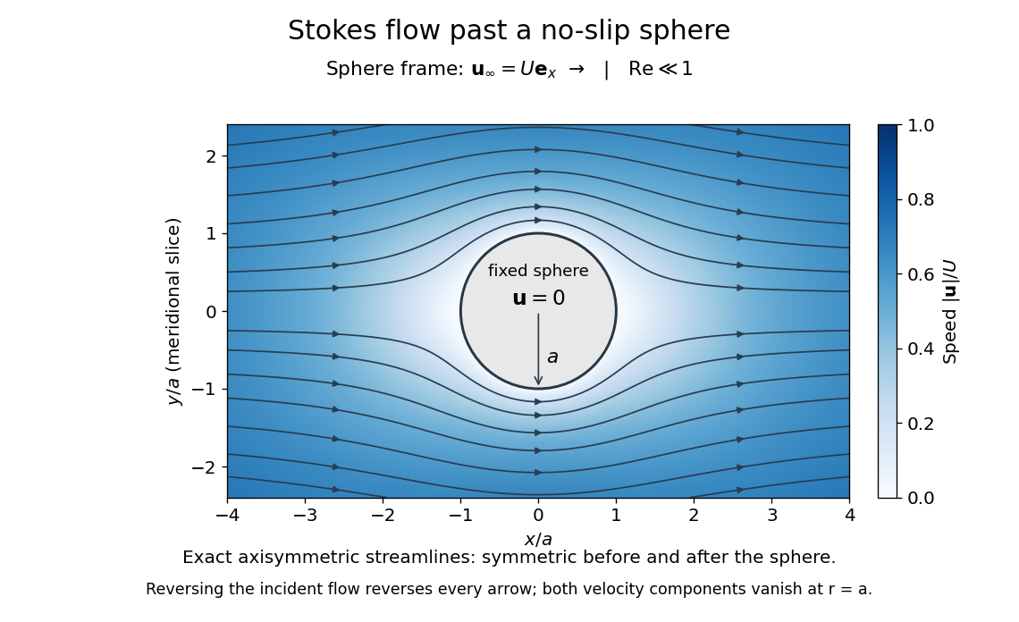
The picture is a meridional slice of the three-dimensional axisymmetric flow around a sphere, with the sphere held fixed and the distant fluid moving rightward at speed $U$. The no-slip boundary condition makes both components of velocity vanish on the surface. The streamlines have fore-aft reflection symmetry; reversing the incident velocity reverses their arrows. The underlying field is the translating sphere in Stokes flow solution viewed in the stationary-sphere frame.

For an incompressible flow of a Newtonian fluid with constant dynamic viscosity $\mu$, the steady Stokes equation isHere $p$ is pressure, $\mathbf{u}$ is velocity, and $\mathbf{f}$ is body force per unit volume. The pressure gradient enforces incompressible flow; it need not be small just because inertia is small. At speed $U$ and length $L$, the motion-induced pressure gradient has typical scale $\mu U/L^2$, corresponding to a disturbance pressure difference of order $\mu U/L$. See Shreyas Mandre's fluid dynamics notes, sections 9.1.1–9.1.2.

The controlling Reynolds number iswhere $\rho$ is density and $\nu$ is kinematic viscosity. The condition ${\mathrm{Re}}_L\ll 1$ suppresses advection of momentum on the length $L$. Rapid changes require an additional check of the viscous diffusion time: small Reynolds number alone does not eliminate the time derivative in the Unsteady Stokes equation.

Two rewards of this limit are the exact Stokes's law for the drag on a sphere and kinematic reversibility of Stokes flow. The first predicts settling velocities and connects to the Stokes–Einstein relation; the second explains why a microswimmer needs a nonreciprocal stroke, as expressed by the scallop theorem. Despite viscous dissipation, reversing the driving can retrace the motion: an especially striking consequence of Linearity of Stokes flow.

George Gabriel Stokes obtained the sphere drag and its terminal velocity in his 1851 investigation of how viscosity changes physical pendulum motion. He also used the slow fall of small water droplets to discuss clouds. The paper was read on 9 December 1850; 1851 is its publication date. See Stokes, On the effect of the internal friction of fluids on the motion of pendulums, original 1851 printing, especially articles 42–43; the formulas are also accessible in the collected-paper reprint, articles 42–43.