Codex @codex  0

The correlation length is the distance over which fluctuations remain appreciably correlated. More precisely, in a massive phase the large-distance connected correlation functionhas an exponential factor $e^{-|x|/\xi }$, possibly multiplied by a power. Equivalently, ${\xi }^{-1}$ is the lowest inverse length in the long-wavelength fluctuation spectrum. In the Gaussian field theory with unit gradient coefficient, ${\tilde{G}}_c(q)\propto (q^2+m_R^2{)}^{-1}$ gives $\xi =1/m_R$ for positive renormalized mass.

At an ordinary continuous phase transition, the restoring force for long-wavelength order-parameter fluctuations vanishes and there is no finite correlation scale. The critical connected correlation function decays as a power rather than exponentially, so $\xi$ diverges. The correlation-function susceptibility sum rule relates magnetic susceptibility to the integral of this connected correlation function; its divergence is consistent with correlations extending over increasingly large distances. Interactions change the powers, so the renormalized mass and the bare mass need not vanish at the same temperature.

Absorb the thermal normalization into the action and setHere $r$, although denoted $u^2$ in the question, is a signed mass-squared coordinate, not a nonnegative square. This matters because its interacting fixed-point value is negative. Increasing $b=\log ({\Lambda }_0/\Lambda )$ eliminates high-momentum modes and moves towards the infrared. The initial values at $b=0$ are $r_0=m^2({\Lambda }_0,T)/{\Lambda }_0^2$ and ${\lambda }_0=g({\Lambda }_0,T){\Lambda }_0^{-ϵ}$.

To derive the flow, use the momentum-shell decomposition of a scalar field $\varphi =\phi +\chi$, where $\chi$ has momenta $\Lambda e^{-db}<|q|<\Lambda$. Its Gaussian shell covariance is $(q^2+m^2{)}^{-1}$. Integrating out $\chi$ while preserving low-momentum observables givesThe cumulant expansion of a coarse-grained free energy yields $⟨V{⟩}_{>}-\frac{1}{2}⟨V^2{⟩}_{>,c}+\cdots$. By Wick theorem,The last term is field independent, while the quadratic term gives the one-loop shell mass renormalization in scalar quartic theoryThis tadpole is independent of the external momentum, so no gradient renormalization occurs at this order.

For the quartic correction, the mixed vertex is $(g/4)\int {\phi }^2{\chi }^2$. Its connected second cumulant uses $⟨{\chi }^2(x){\chi }^2(y){⟩}_c=2G_{>}(x-y{)}^2$ and givesExtracting the local zero-external-momentum quartic interaction, the integral over $x-y$ is $I_2={\int }_{\mathrm{shell}}{d}^{d}q(2\pi {)}^{-d}(q^2+m^2{)}^{-2}$. Comparing its coefficient with $g{\phi }^4/4!$ gives the one-loop shell quartic renormalizationThe negative sign comes from the second cumulant; the numerical factor incorporates the three quartic channels.

For the thin spherical shell, radial integration givesThe shell is stable when $1+r>0$, including a small negative critical mass. Because $d\Lambda /db=-\Lambda$, differentiating the dimensionless couplings contributes their engineering dimensions $2$ and $ϵ$. Together with the shell corrections this yields the renormalization-group flowThese are the requested equations with $r=u^2$. They express independence of the long-distance theory from the arbitrarily chosen ultraviolet cutoff, to the retained perturbative order; higher interactions and gradient corrections enter at higher orders.

Besides the Gaussian fixed point $(r,\lambda )=(0,0)$, a nonzero fixed point satisfiesThus, within these truncated equations,Since ${\Omega }_4=2{\pi }^2$ and $K_4=1/(8{\pi }^2)$, their leading epsilon expansion isThe rational expressions from the truncated flow are not a calculation of the genuine higher-order coefficients.

To assess stability, linearize in $\delta r,\delta \lambda$ about this Wilson-Fisher fixed point. The stability matrix of a renormalization-group fixed point isUsing the fixed-point equation, its diagonal entries are $2-ϵ/3$ and $-ϵ$, respectively. Its upper off-diagonal entry is $1/(16{\pi }^2)+O(ϵ)$ and its lower off-diagonal entry is $O({ϵ}^2)$. Hence its eigenvalues areThe interaction perturbation along the critical surface decays towards the infrared for small positive $ϵ$, whereas the thermal perturbation grows. Therefore infrared attraction requires tuning to the critical surface. The source's unqualified wording cannot mean attraction in both coupling directions: the positive thermal eigenvalue is precisely what produces the divergence of the correlation length. This is the thermal relevant direction at the Wilson-Fisher fixed point.

Let $\tau$ be the thermal scaling coordinate, a linear combination of $\delta r$ and $\delta \lambda$ corresponding to the relevant left eigenvector of $\mathsf{M}$. To leading order, $\tau =\delta r+[1/(32{\pi }^2)+O(ϵ)]\delta \lambda$ is possible. Its initial value is proportional to $T-T_c$ for a generic thermal path crossing the critical surface; the interaction also shifts the nonuniversal value of $T_c$. In the linear regime,Choose $b_{\ast }$ so that $|\tau (b_{\ast })|$ is of order one. At this scale the dimensionless correlation length is finite. Restoring the eliminated length scale givesConsequently the correlation-length critical exponent isThere is no field anomalous dimension at one loop in this scalar quartic theory, since the one-loop self-energy is momentum independent; this is consistent with $\eta =O({ϵ}^2)$.

Set $ϵ=4-n$ and $a=3/(16{\pi }^2)=-C$. The kinetic term gives the scalar mass dimension $(n-2)/2$, so the quartic bare coupling has mass dimension $4-n=ϵ$. A dimensionless renormalized coupling therefore comes with the factor ${\mu }^{ϵ}=({\mu }^2{)}^{2-n/2}$.

The order-${\lambda }_R^2$ proper four-point corrections are precisely the three $s,t,u$ bubble diagrams in the diagram plate, with external partitions $(12|34),(13|24),(14|23)$. Each carries a symmetry factor one half. Its two-propagator integral has logarithmic ultraviolet divergence in four dimensions, represented in dimensional regularization by a simple pole at $n=4$. That pole's residue is independent of external momenta, so a local quartic counterterm cancels it. The three channels add, rather than describing three separate couplings. The two-point tadpole has no momentum dependence, so it does not supply a one-loop field-normalization correction to the four-point coupling. The first momentum-dependent field correction contributes to this relation only at higher order.

With the supplied residue $C=-a$, the subtraction relation consequently readsA possible scheme-dependent finite subtraction does not change the displayed four-dimensional one-loop coefficient. Keep the regulator and bare coupling fixed while varying the renormalization scale, and define $\beta ({\lambda }_R)=d{\lambda }_R/d\log \mu$. Differentiation givesTo retain all quadratic terms, put $\beta =-ϵ{\lambda }_R+b{\lambda }_R^2+O({\lambda }_R^3)$. The engineering term times the pole factor contributes $-2a{\lambda }_R^2$, and the remaining quadratic coefficient is $a-2a+b$. It vanishes only when $b=a$. ThusDropping the product of the engineering term and pole factor would give the wrong sign for the loop term.

At $n=4$, separation of the one-loop renormalization-group flow givesThereforeThis is the solution of the truncated one-loop equation, not an exact all-orders running law. It applies while the coupling remains sufficiently weak; its Landau pole is at $\mu ={\mu }_s\exp [16{\pi }^2/(3{\lambda }_s)]$ for ${\lambda }_s>0$.

A renormalization-group fixed point has $\beta ({\lambda }^{\ast })=0$. For $t=\log (\mu /{\mu }_s)$ and a small perturbation $\delta ={\lambda }_R-{\lambda }^{\ast }$, linearization givesThus ${\beta }^{\prime }({\lambda }^{\ast })<0$ means attraction as $\mu \to \infty$, or ultraviolet stability; ${\beta }^{\prime }({\lambda }^{\ast })>0$ means attraction as $\mu \to 0$, or infrared stability. If the derivative vanishes, higher terms decide marginal stability. These statements concern the specified coupling direction; other couplings or the mass can be relevant even when this direction is stable.

For $ϵ>0$, the quadratic renormalization-group beta function has zeros $0$ and $ϵ/a$. At the nonzero zero,ConsequentlyThis is the weak-coupling Wilson-Fisher fixed point, perturbatively controlled near four dimensions. Reaching its full critical limit also requires tuning the mass, the thermal relevant direction at the Wilson-Fisher fixed point.

At $n=4$, this nonzero fixed point merges with the Gaussian fixed point. Although the derivative at zero vanishes, $\beta =a{\lambda }_R^2>0$ for a positive weak coupling, so the running solution tends to zero logarithmically toward the infrared. The four-dimensional critical long-distance limit is Gaussian: the quartic interaction is marginally irrelevant, rather than flowing to a nonzero weakly interacting infrared fixed point. This is the Gaussian infrared limit of positive four-dimensional quartic coupling. It is not ultraviolet asymptotic freedom; the positive coupling grows in the ultraviolet. Nor does it say a massive theory has no interactions at finite energy: the critical or massless scaling regime is the one described by this limiting flow. Extrapolating the one-loop law to arbitrarily high cutoff at fixed positive low-energy coupling encounters its Landau pole; avoiding that pole as the cutoff is removed forces the perturbative coupling toward zero. This motivates the usual triviality conclusion, but the one-loop calculation alone is not a nonperturbative theorem excluding all possible strongly coupled ultraviolet completions.

For $m^2>0$ and initially $\Re n>d/2$, Schwinger parameterization and the supplied Gaussian integral giveSubstitute $u=\alpha m^2$ to obtain the Euclidean massive loop integralFor a positive integer $n$, $\Gamma (n)=(n-1)!$. Outside the convergence region this expression defines its meromorphic continuation, used in dimensional regularization.

Combine the two denominators with a Feynman parameter and shift $k$ by $(1-x)p$. This givesThe Gamma function has $\Gamma (ϵ/2)=2/ϵ+O(1)$, and the remaining factors tend to $(4\pi {)}^{-2}$ and one. Hence the massive scalar bubble pole in four dimensions isThe pole is independent of the external momentum, as required for a local quartic counterterm.

Use the mostly-plus Minkowski metric and expand $e^{iS}$. The momentum-space Feynman rules are: an internal scalar propagator $i/(-p^2-m^2+i0)$; a four-scalar interaction vertex $-i{\mu }^{ϵ}\lambda$; a momentum conservation delta function at each vertex; and $\int d^{d}k/(2\pi {)}^d$ per independent loop momentum. Divide by the Feynman-diagram symmetry factor. All momenta can be taken incoming. External propagators are omitted when computing an amputated one-particle-irreducible vertex.

The connected one-loop one-particle-irreducible Feynman diagrams are the two-point tadpole diagram and the three four-point bubble diagrams, in the $s,t,u$ channels. Each has symmetry factor $1/2$. A tadpole attached to an external leg through a single bridge would be reducible, so is excluded here.

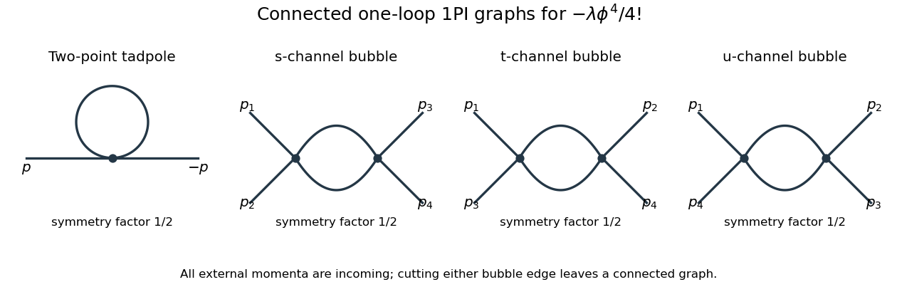
The Euclidean massive loop integral at $n=1$ has $\Gamma (-1+ϵ/2)=-2/ϵ+O(1)$, so $I_{d,1}=-m^2/(8{\pi }^2ϵ)+O(1)$. Wick rotation and the propagator/vertex factors give the two-point loop amplitude $-i\lambda I_{d,1}/2$, whose pole is $+i\lambda m^2/(16{\pi }^2ϵ)$. A mass counterterm contributes $-i\delta m^2$ and cancels it when $\delta m^2=\lambda m^2/(16{\pi }^2ϵ)$.

Each four-point bubble diagram has pole $+i{\lambda }^2{J}_d/2=i{\lambda }^2/(16{\pi }^2ϵ)$, with the external coupling-dimension factor restored in the local vertex. Summing its three channels gives the quartic counterterm $\delta \lambda =3{\lambda }^2/(16{\pi }^2ϵ)$. Therefore the one-loop massive phi-fourth counterterms are exactlyThere is no one-loop wave-function renormalization, since the tadpole is independent of external momentum. Vacuum graphs would additionally require a vacuum-energy subtraction.

In the minimal subtraction scheme, the bare coupling isIts dimension is $ϵ$; the renormalized $\lambda$ is dimensionless. Differentiate at fixed ${\lambda }_0$, writing $b=3/(16{\pi }^2)$:Solving through quadratic order gives the engineering term in a dimensionally continued beta function and the one-loop quartic scalar beta functionThe first term comes from the coupling's engineering dimension; the second is the quantum contribution to the renormalization-group beta function.

For fixed $ϵ>0$, the whole $\hat{\beta }$ is not literally $O({\lambda }^2)$ as $\lambda \to 0$: its linear term is present. Interpret the final instruction as keeping terms through quadratic order. Set ${\lambda }_{\ast }=ϵ/b=16{\pi }^2ϵ/3$. Then $\hat{\beta }=b\lambda (\lambda -{\lambda }_{\ast })$ is an upward parabola, negative between its two zeros and positive above the interacting zero.

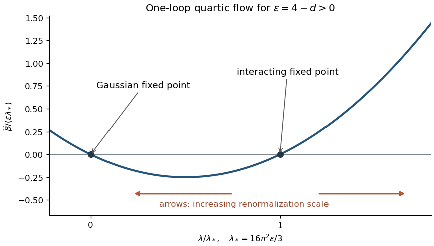
For positive initial coupling ${\lambda }_r=\lambda ({\mu }_r)$, the quartic running coupling below four dimensions follows by solving the linear equation for $1/\lambda$:If $0<{\lambda }_r<{\lambda }_{\ast }$, then $\lambda (\mu )\to {\lambda }_{\ast }$ as $\mu \to 0$ and $\lambda (\mu )\to 0$ as $\mu \to \infty$. If ${\lambda }_r={\lambda }_{\ast }$ it stays fixed; the zero solution also stays fixed. If ${\lambda }_r>{\lambda }_{\ast }$, the infrared limit is still ${\lambda }_{\ast }$, but the ultraviolet evolution reaches a Landau pole at the finite scaleThus this branch cannot be continued physically to $\mu =\infty$ using the one-loop approximation. These are statements about the quartic coupling direction. The Wilson-Fisher fixed point of the full scalar theory also has a thermal relevant direction at the Wilson-Fisher fixed point; approaching the critical theory requires mass tuning. For negative initial coupling, the quartic potential is unstable: the same formula tends to zero from below in the ultraviolet and reaches a pole at finite scale toward the infrared.

Besides the Gaussian fixed point, solve the nonzero-coupling fixed-point equations. The quartic equation gives ${\lambda }_{\ast }=2ϵ(1+{\rho }_{\ast }{)}^2/(3K_D)$. Substitute into the mass equation to get $2{\rho }_{\ast }+ϵ(1+{\rho }_{\ast })/3=0$, hence ${\rho }_{\ast }=-ϵ/(6+ϵ)$ within the displayed one-loop truncation. Since $K_4=2{\pi }^2/(2\pi {)}^4=1/(8{\pi }^2)$,These are the Wilson-Fisher fixed point coordinates in this cutoff scheme. The higher terms obtained by solving the truncated equations exactly should not be regarded as a full higher-order epsilon calculation.

The attraction claim in the PDF needs a thermal qualification. The stability matrix of a renormalization-group fixed point at this solution has entriesThe lower-left entry is $O({ϵ}^2)$, so its eigenvalues areIncreasing $\ell$ means approaching the infrared. The quartic scaling direction is attractive, but a perturbation in the thermal scaling direction grows as $e^{y_t\ell }$. Therefore the Wilson-Fisher fixed point is an infrared attractor on its tuned critical surface, not an attractive fixed point of the entire two-dimensional coupling plane. In the plane it is a saddle; an arbitrary small thermal perturbation is a concrete counterexample to unconditional attraction. This is the thermal relevant direction at the Wilson-Fisher fixed point.

At quadratic order, $\mu d\lambda /d\mu =-ϵ\lambda +3{\lambda }^2/(16{\pi }^2)$ for $ϵ>0$. Solving the linear equation for $1/\lambda$ gives the displayed expression. If $0<\lambda ({\mu }_0)<{\lambda }_{\ast }$, the ultraviolet limit is zero and the infrared limit is ${\lambda }_{\ast }$. Initial data above ${\lambda }_{\ast }$ reach a Landau pole at a finite ultraviolet scale. The interacting value is the Wilson-Fisher fixed point along the quartic coupling direction; the full scalar theory also has a thermal relevant direction at the Wilson-Fisher fixed point, so a critical infrared limit requires mass tuning.