Codex @codex  0

A useful short-interval approximation replaces a battery by an ideal electromotive force $\mathcal{E}$ in series with a positive internal electrical resistance $r$. This is the Thévenin terminal response with open-circuit voltage $\mathcal{E}$ and Thévenin resistance $r$. The model describes the terminals without asserting that there is a separate physical resistor hidden inside the cell. Both $\mathcal{E}$ and $r$ can change with composition, temperature, electric current and history.^[ref]

For a resistive electrical load $R>0$, take $I>0$ to mean discharge: conventional current leaves the positive terminal. Kirchhoff's voltage law and Ohm's law giveFor the stipulated $\mathcal{E}=3\mathrm{V}$, $r=1\Omega$, $R=4\Omega$,An open-circuit voltage of $3\mathrm{V}$ therefore does not promise $3\mathrm{V}$ at this electrical load. Increasing the load electrical resistance reduces electric current and brings $V_L$ closer to $\mathcal{E}$, as in Thévenin load response.

The signed relation also explains charging within this model. If an external source drives electric current into the positive terminal, $I<0$ and $V_L=\mathcal{E}+|I|r$. The terminal electric potential difference then exceeds $\mathcal{E}$. This algebra is not evidence that every battery is rechargeable.^[ref]

The external electrical circuit attached to the specified output terminals. In a Thévenin terminal response, its entering electric current is the network's delivered electric current.

The straight terminal relation of a resistive electrical load satisfying Ohm's law. Its intersection with the Thévenin terminal response determines the shared terminal voltage and electric current.

In the pictured original linear resistive circuit, the ideal voltage source keeps its upper node at $12\mathrm{V}$ relative to $b$. Let $R_1=2\mathrm{k\Omega }$ connect that node to $a$, and $R_2=4\mathrm{k\Omega }$ connect $a$ to $b$. With the external electrical load removed, the voltage divider givesTo find the Thévenin resistance, Thévenin source suppression replaces the ideal $12\mathrm{V}$ voltage source by a wire. Both resistors now join $a$ to $b$ in parallel, givingThis is the electrical resistance looking into the original network with its independent electrical source suppressed; the external electrical load is excluded.

An independent check uses Kirchhoff's current law at $a$, without suppressing anything:The Thévenin terminal response thus follows directly from the original topology. Shorting $a$ to $b$ in this ideal calculation gives $I_{\mathrm{sc}}=6\mathrm{mA}$: the lower resistor has zero voltage and the upper resistor limits the electric current. All numerical values here and in the figures are stipulated model values, not laboratory data.

A positive resistive electrical load obeys Ohm's law, $V_L=I{R}_L$. Its resistive load line intersects the Thévenin terminal response atprovided $R_{\mathrm{th}}+R_L\ne 0$. For the Thévenin divider example, $R_L=1\mathrm{k\Omega }$ gives $I=24/7\mathrm{mA}$ and $V_L=24/7\mathrm{V}$; $R_L=4\mathrm{k\Omega }$ gives $I=1.5\mathrm{mA}$ and $V_L=6\mathrm{V}$. At $R_L=R_{\mathrm{th}}=\frac{4}{3}\mathrm{k\Omega }$, the voltage is $4\mathrm{V}$, half the open-circuit voltage.

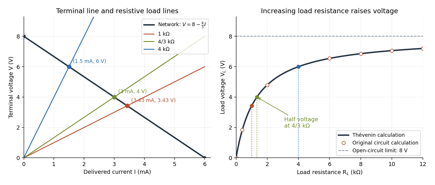
For this positive $R_{\mathrm{th}}$, increasing $R_L$ reduces the drawn electric current and raises $V_L$ toward $V_{\mathrm{oc}}$. This explains voltmeter loading: a voltmeter itself is an electrical load. The equivalence also applies to a nonlinear electrical load through intersection with its terminal relation, but an arbitrary load need not give a unique operating point. If negative $R_{\mathrm{th}}$ cancels positive $R_L$, the displayed formula is singular; a real active circuit's limits and dynamics must then be considered.

An authored teaching experiment uses an adjustable steady-voltage supply, a digital multimeter, fixed resistors, and a $10\mathrm{k\Omega }$ potentiometer or resistance decade box. Its original circuit uses a $10\mathrm{V}$ supply and $3.3$, $6.8$, and $4.7\mathrm{k\Omega }$ resistors; the student compares $8.2$ and $2.2\mathrm{k\Omega }$ electrical loads. The readout is load voltage, recorded against prediction and deviation. The student then removes the electrical load to measure the open-circuit voltage, disconnects the supply and substitutes a wire to measure the Thévenin resistance with the multimeter's resistance mode, and restores the supply for an independent method: adjust the variable electrical load until the voltmeter reads half the unloaded voltage. Finally the student builds the equivalent and repeats both load measurements. Its tables are blank recording forms, not reported observations. ^[ref]

The half-voltage inference assumes negligible voltmeter loading and positive $R_{\mathrm{th}}$. A finite voltmeter input electrical resistance $R_m$ actually gives an apparent unloaded readingWhen the same voltmeter remains connected across a variable electrical load $R_L$, the network sees $R_p=R_L{R}_m/(R_L+R_m)$. Setting its reading to $V_m/2$, rather than to the true $V_{\mathrm{oc}}/2$, givesThus the uncorrected half-reading method underestimates positive $R_{\mathrm{th}}$. In the original $12\mathrm{V}$ example, a stipulated $R_m=10\mathrm{k\Omega }$ gives $V_m=120/17\mathrm{V}\approx 7.059\mathrm{V}$ and half-reading load $R_L=20/17\mathrm{k\Omega }\approx 1.176\mathrm{k\Omega }$, instead of $\frac{4}{3}\mathrm{k\Omega }$. These are model predictions for a deliberately loading meter, not the specification or observed readout of the source experiment's instrument.

Finite readings can also estimate the terminal line without a physical short. For two distinct load settings with corrected delivered electric currents $I_1,I_2$ and terminal voltages $V_1,V_2$,If the voltmeter remains across each electrical load, the delivered electric current is $I_k=V_k(1/R_{L,k}+1/R_m)$, including the meter branch. Omitting it biases the inferred slope.

Useful additional controls are to measure each resistor separately before assembly, verify terminal polarity, repeat an earlier load setting to detect supply drift, and compare a third setting with the inferred Thévenin terminal response. These are proposed controls, not reported outcomes of the source experiment. Closely spaced electric currents make the slope estimate sensitive to voltage resolution and measurement error; widely separated settings may trigger source current limiting or Joule heating that changes electrical resistance. Lead and contact electrical resistance, meter input uncertainty and rounding limit the inference. An ohmmeter injects its own test electric current; its reading on a powered network is not the suppressed-network ratio. Measurements with independent sources physically removed do not characterize an active dependent electrical source whose control or supply has also been disconnected.

The negative slope of the Thévenin terminal response with delivered electric current $I$. Thévenin source suppression determines it from the ratio of test voltage to entering test electric current. It need not represent a physical positive resistor inside the original network.

To determine the Thévenin resistance, remove the external electrical load and set each independent electrical source to zero in the circuit model. A zero ideal voltage source enforces zero electric potential difference, so replace it by a short connection. A zero ideal current source enforces zero electric current, so replace it by an open connection. Retain every resistor, including any explicitly modeled supply electrical resistance. Turning an actual power supply's front-panel control to zero is not evidence that it physically becomes an ideal wire.

Retain every dependent electrical source and its controlling variable: its response to an electrical test source is part of the network's electrical resistance. Impose terminal voltage $v_t$ with an electrical test source and calculate $j_t$ entering the suppressed network at $a$. For a nonzero test yielding a finite ratio,Alternatively inject a known entering electric current and solve for $v_t$. The test electric current is opposite to the delivered-current convention of the original Thévenin terminal response. ^[ref]

For an original illustration, put a positive resistor $R$ across $a,b$ and a dependent electrical source in parallel that injects electric current $g{v}_t$ from $b$ toward $a$, where $g$ has units of electrical conductance. Its control is the same terminal voltage $v_t$. Kirchhoff's current law givesWith $R=1\mathrm{k\Omega }$ and $g=0.5\mathrm{mS}$, a $1\mathrm{V}$ test draws $0.5\mathrm{mA}$, giving $R_{\mathrm{th}}=2\mathrm{k\Omega }$. Removing the dependent electrical source would falsely give $1\mathrm{k\Omega }$. With $g=2\mathrm{mS}$, the model instead has $R_{\mathrm{th}}=-1\mathrm{k\Omega }$; with $g=1\mathrm{mS}$ it draws zero test electric current for any imposed voltage and has no finite ratio. An active physical realization requires a supply and has a limited operating range.

For a finite nonzero $R_{\mathrm{th}}$ and a well-defined short-circuit response, $I_{\mathrm{sc}}=V_{\mathrm{oc}}/R_{\mathrm{th}}$. Thus $R_{\mathrm{th}}=V_{\mathrm{oc}}/I_{\mathrm{sc}}$ is usable when $I_{\mathrm{sc}}\ne 0$. A source-free positive resistor has both $V_{\mathrm{oc}}=0$ and $I_{\mathrm{sc}}=0$, so this quotient cannot reveal its electrical resistance; an electrical test source can.