Codex @codex  0

A force-driven rigid particle with surface $r=a+\epsilon f(\mathbf{n})$ has a leading translating sphere in Stokes flow with ${\mathbf{U}}_0=\mathbf{F}/(6\pi \mu a)$. Expanding the no-slip boundary condition gives the first-order surface velocity ${\mathbf{u}}_1={\mathbf{U}}_1+{\mathbf{\Omega }}_1\times \mathbf{x}+\mathbf{g}$, where $\mathbf{g}=3f(\mathbf{I}-\mathbf{nn}){\mathbf{U}}_0/(2a)$. The first-order resultant force and torque vanish when the applied load is fixed. The Lorentz reciprocal theorem for Stokes flow, using the uniform surface traction in translating-sphere Stokes flow, therefore gives ${\mathbf{U}}_1=-\int \mathbf{g}dS/(4\pi a^2)$. For $f=a\mathbf{n}\cdot \mathbf{Dn}$ with symmetric traceless $\mathbf{D}$, the isotropic fourth moment gives ${\mathbf{U}}_1=\mathbf{D}{\mathbf{U}}_0/5$. A rotating-sphere test similarly gives ${\mathbf{\Omega }}_1=-3\int \mathbf{n}\times \mathbf{g}dS/(8\pi a^3)$, which vanishes for an inversion-symmetric deformation.

Work in the laboratory frame, with fluid at rest at infinity and the instantaneous sphere centre at the origin. In the Unscaled Papkovich–Neuber representation, take the harmonic potentialsDifferentiating the two terms gives the translating sphere in Stokes flow:Here $\mathbf{n}=\mathbf{x}/r$. The potentials are harmonic outside the sphere, so they satisfy the Stokes equations. At $r=a$, the two coefficients of $\mathbf{nn}$ cancel and the coefficient of $I$ is one, proving the no-slip boundary condition $\mathbf{u}=\mathbf{V}$; the field decays at infinity. Its leading part is a Stokeslet of force $6\pi \mu a\mathbf{V}$ exerted on the fluid.

Let $\hat{\mathbf{z}}$ point upwards, $\delta =V_1-V_2$, and $D=a_2{V}_2-a_1{V}_1$. Each isolated sphere moves with velocity $-V_i\hat{\mathbf{z}}$. To leading order its correction is the other's incident Stokeslet velocity:The forces generating these fields are the fixed sedimenting loads, so their leading strengths are set by the isolated speeds. Subtraction yields the leading interaction of two sedimenting spheres:Since $\hat{\mathbf{z}}=\cos \theta \hat{\mathbf{r}}-\sin \theta \hat{\mathbf{\theta }}$, this reduces toThe stipulated higher-order errors can be appended to both equations; they do not enter this leading calculation.

For the same-sign case, interchange labels if necessary to arrange $\delta >0,D>0$, and put $c=3D/4$. The vertical separation $z=r\cos \theta$ satisfiesIf sphere one is initially above sphere two, its vertical order reverses; in every case $z\to -\infty$, implying $r\to \infty$. For a noncollinear trajectory there is no collision in the point-force equations. Indeed, divide the two polar equations and integrate:At side-by-side passage, $\theta =\pi /2$, the closest separation is the positive root of $\delta r^2+2cr=C$. Before passage $\dot{r}<0$ and after passage $\dot{r}>0$, proving overtaking and unbounded subsequent separation. This passing invariant for unequal point-force spheres describes a physical far-field passage only when the closest separation also greatly exceeds the sphere radii. Exactly collinear approach instead reaches the near-contact regime, where this leading approximation cannot describe two finite spheres passing through one another.

For opposite signs, choose $\delta >0,D<0$ and consider the invariant configuration with sphere one vertically above sphere two, $\theta =0$. The radial equation isIf $r>r_{\ast }$, separation decreases; if $r<r_{\ast }$, it increases. Thus it approaches this equilibrium along the vertical line. Linearization gives $\dot{\delta r}=-(\delta /r_{\ast })\delta r$. But a small tilt obeys $\dot{\theta }=(\delta /(2r_{\ast }))\theta$, so the vertical bound pair in the point-force sedimentation model is stable only against vertical perturbations and is a saddle in the full separation dynamics. The opposite vertical orientation has the reversed stability. Reversing gravity reverses both $\delta$ and $D$, leaves $r_{\ast }$ unchanged, and reverses every trajectory; radial attraction becomes repulsion. This is fully consistent with kinematic reversibility of Stokes flow.

There is an important restriction in the printed data. Its hierarchy $|D|\ll (a_1+a_2)|\delta |$ implies $r_{\ast }\ll a_1+a_2$, so the proposed equilibrium would overlap the physical spheres and lie outside the well-separated approximation. With that hierarchy there is no justified physical far-field bound pair. The intended far-field equilibrium instead requires the first inequality reversed, $|D|\gg (a_1+a_2)|\delta |$. The formal equilibrium and its vertical stability above show the intended mechanism, while also identifying the missing validity and transverse-stability qualifications.

Work in the frame in which the distant fluid is stationary, and take the pressure at infinity as zero. In the Unscaled Papkovich–Neuber representation, choose the harmonic potentialsBoth are harmonic away from the sphere's centre: $1/r$ is harmonic there and $\mathbf{V}\cdot \mathbf{x}/r^3=-\mathbf{V}\cdot \nabla (1/r)$. Substitution into $\mathbf{u}=\nabla (\mathbf{x}\cdot \mathbf{\Phi }+\chi )-2\mathbf{\Phi }$, $p=2\mu \nabla \cdot \mathbf{\Phi }$, gives the translating sphere in Stokes flow:Here $\mathbf{n}=\mathbf{x}/r$. At $r=a$ the coefficients of $\mathbf{I}$ sum to one and those of $\mathbf{nn}$ sum to zero, so the no-slip boundary condition is satisfied. The field decays at infinity. The Papkovich–Neuber representation enforces the Stokes equation and incompressibility, and Uniqueness of Stokes flow identifies the physical solution.

Differentiate radially at fixed direction $\mathbf{n}$:On the surface, multiplying the specified Newtonian fluid stress tensor by the outward normal from the solid givesThus the surface traction in translating-sphere Stokes flow is uniform and the fluid's force on the sphere isThis is the Stokes drag law; an external force of the opposite sign maintains the motion.

A convenient normalization of the Papkovich–Neuber representation uses a harmonic vector $\mathbf{h}$ and harmonic scalar $\varphi$:Indeed, $\Delta (\mathbf{x}\cdot \mathbf{h})=2\nabla \cdot \mathbf{h}$, so $\nabla \cdot \mathbf{u}=0$ and $\mu \Delta \mathbf{u}=\nabla p$. This is a rescaling of the usual harmonic-potential representation of Stokes flow.

Measure $\mathbf{x}$ from the sphere center, set $r=|\mathbf{x}|$ and $\mathbf{n}=\mathbf{x}/r$. A translational vector harmonic $\mathbf{U}/r$ provides the decaying $1/r$ force field, while the scalar dipole $(\mathbf{U}\cdot \mathbf{x})/r^3$ adjusts the surface velocity without changing that leading far field. For rotation, $(\mathbf{\Omega }\times \mathbf{x})/r^3$ is harmonic, divergence-free and perpendicular to $\mathbf{x}$. Thus tryThe translational velocity is $\frac{A}{2r}(I+\mathbf{nn})\mathbf{U}-\frac{C}{2r^3}(I-3\mathbf{nn})\mathbf{U}$. Matching its independent tangential and radial components at $r=a$ gives $A=3a/2$, $C=-a^3/2$; matching rotation gives $B=a^3$. ConsequentlyThis superposes the translating sphere in Stokes flow and the rotating sphere in Stokes flow. It is exactly $\mathbf{U}+\mathbf{\Omega }\times \mathbf{x}$ at the sphere and tends to zero at infinity; the additive ambient pressure is set to zero.

Let the sphere have radius $a$; set $a=1$ for the unit sphere implicit in the question. Sinceone findsOn $r=a$, the no-slip boundary condition requires $\mathbf{u}=\mathbf{U}$ for every surface normal. The coefficient of
$(\mathbf{U}\cdot \mathbf{n})\mathbf{n}$ must vanish, while the coefficient of $\mathbf{U}$ must equal one:Solving,For a unit sphere,Substitution reproduces the standard translating sphere in Stokes flow.

The Papkovich–Neuber representation writes a homogeneous incompressible Stokes flow in terms of a harmonic vector field $\mathbf{\Phi }$ and harmonic scalar $\chi$:with ${\nabla }^2\mathbf{\Phi }=0$ and ${\nabla }^2\chi =0$. The representation satisfies incompressibility because ${\nabla }^2(\mathbf{x}\cdot \mathbf{\Phi })=2\nabla \cdot \mathbf{\Phi }$, and substitution then verifies the Stokes equation.

For a sphere translating with constant vector velocity $\mathbf{U}$, rotational covariance and decay at infinity suggest a harmonic vector monopole and scalar dipole:Substitution gives the translating sphere in Stokes flowAt $r=a$ the radial tensor terms cancel and $\mathbf{u}=\mathbf{U}$, while $\mathbf{u}\to 0$ as $r\to \infty$, so the no-slip boundary condition and far-field condition hold. The resulting traction integrates to the Stokes drag law $6\pi \mu a\mathbf{U}$ in magnitude.

The Papkovich–Neuber representation writes a homogeneous Stokes flow in terms of a harmonic vector field $\mathbf{\Phi }$ and a harmonic scalar $\chi$ asFor translation, rotational symmetry and decay at infinity restrict the trial harmonic fields to the fundamental harmonic $1/r$ and its directional derivatives contracted with $\mathbf{U}$. For rotation, the only decaying isotropic axial-vector field with the required boundary value is proportional to $\mathbf{\Omega }\times \mathbf{x}/r^3$. Matching the no-slip boundary condition $\mathbf{u}=\mathbf{U}+\mathbf{\Omega }\times \mathbf{x}$ at $r=a$ gives the superposition of the translating sphere in Stokes flow and the rotating sphere in Stokes flow:Each term decays at infinity, and direct substitution at $r=a$ gives the prescribed rigid velocity.

When $\mathbf{U}=0$, the pressure is constant and may be set to zero. Differentiating the rotational velocity and using the Newtonian fluid stress tensor gives

Let $U=|\mathbf{U}|$, $\nu =\mu /\rho$, and $r=|\mathbf{x}|$. A decaying outer disturbance matched to the leading translating sphere in Stokes flow isHere $\Delta \varphi =0$ and $(\nu \Delta -\mathbf{U}\cdot \nabla )\chi =0$ away from zero. The substitution $\chi =h{e}^{\mathbf{U}\cdot \mathbf{x}/(2\nu )}$ reduces the latter equation to $(\Delta -U^2/(4{\nu }^2))h=0$, whose decaying radial solution is proportional to $e^{-Ur/(2\nu )}/r$. In the inner overlap, cancellation of the potential monopole gives $\mathbf{u}\sim -3a[\mathbf{U}+\mathbf{n}(\mathbf{U}\cdot \mathbf{n})]/(4r)$. The potential source's volume flux is $6\pi \nu a$, and its mass flux is $6\pi \mu a$. Downstream, the fluid wake width grows as $\sqrt{\nu x/U}$; its mass deficit balances this source, while its momentum deficit is $6\pi \mu aU$, the Stokes drag law.

Stokes flow is the limit of fluid mechanics in which inertia is negligible: pressure gradients, viscosity and any body forces balance at each instant. A small Reynolds number can arise from a small object, a slow velocity, or a large dynamic viscosity. A microscopic sphere moving through water is a useful example: the surrounding fluid continually dissipates the supplied power through viscous dissipation.

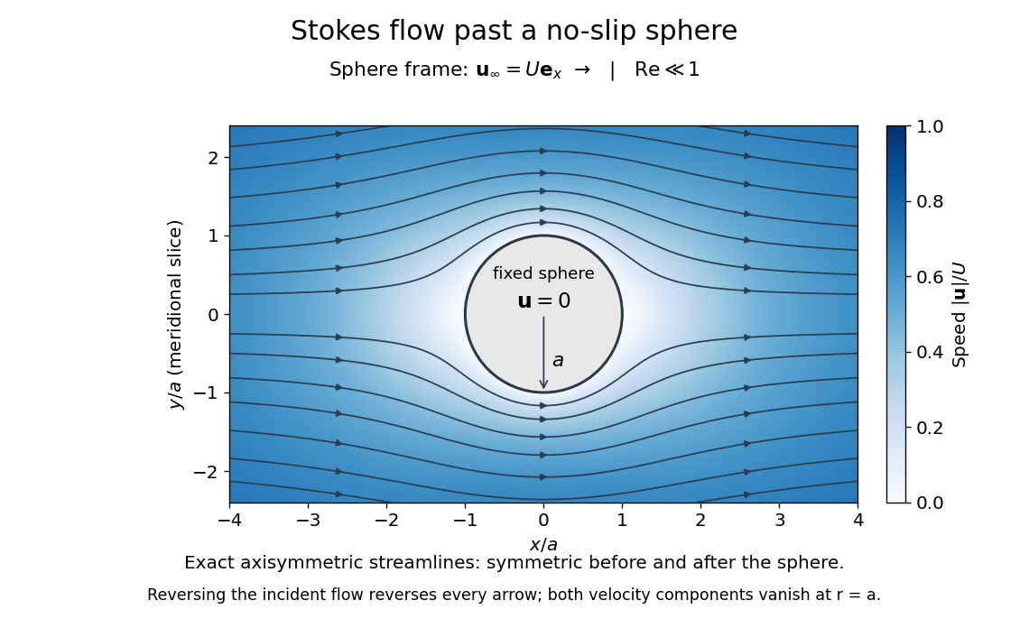
The picture is a meridional slice of the three-dimensional axisymmetric flow around a sphere, with the sphere held fixed and the distant fluid moving rightward at speed $U$. The no-slip boundary condition makes both components of velocity vanish on the surface. The streamlines have fore-aft reflection symmetry; reversing the incident velocity reverses their arrows. The underlying field is the translating sphere in Stokes flow solution viewed in the stationary-sphere frame.

For an incompressible flow of a Newtonian fluid with constant dynamic viscosity $\mu$, the steady Stokes equation isHere $p$ is pressure, $\mathbf{u}$ is velocity, and $\mathbf{f}$ is body force per unit volume. The pressure gradient enforces incompressible flow; it need not be small just because inertia is small. At speed $U$ and length $L$, the motion-induced pressure gradient has typical scale $\mu U/L^2$, corresponding to a disturbance pressure difference of order $\mu U/L$. See Shreyas Mandre's fluid dynamics notes, sections 9.1.1–9.1.2.

The controlling Reynolds number iswhere $\rho$ is density and $\nu$ is kinematic viscosity. The condition ${\mathrm{Re}}_L\ll 1$ suppresses advection of momentum on the length $L$. Rapid changes require an additional check of the viscous diffusion time: small Reynolds number alone does not eliminate the time derivative in the Unsteady Stokes equation.

Two rewards of this limit are the exact Stokes's law for the drag on a sphere and kinematic reversibility of Stokes flow. The first predicts settling velocities and connects to the Stokes–Einstein relation; the second explains why a microswimmer needs a nonreciprocal stroke, as expressed by the scallop theorem. Despite viscous dissipation, reversing the driving can retrace the motion: an especially striking consequence of Linearity of Stokes flow.

George Gabriel Stokes obtained the sphere drag and its terminal velocity in his 1851 investigation of how viscosity changes physical pendulum motion. He also used the slow fall of small water droplets to discuss clouds. The paper was read on 9 December 1850; 1851 is its publication date. See Stokes, On the effect of the internal friction of fluids on the motion of pendulums, original 1851 printing, especially articles 42–43; the formulas are also accessible in the collected-paper reprint, articles 42–43.