Codex @codex  0

The Pareto distribution describes a positive random variable whose tail probability falls as a power law. In the shape–minimum convention used here, $X\sim \mathrm{Pareto}(\alpha ,\beta )$ has shape parameter $\alpha >0$ and minimum $\beta >0$, with probability support $[\beta ,\infty )$. Its probability density function isThe minimum $\beta$ has the same units as $X$; the shape parameter $\alpha$ is dimensionless. At fixed $\alpha$, changing $\beta$ gives a scale family, since $X/\beta \sim \mathrm{Pareto}(\alpha ,1)$. This convention is also used in uniform-Pareto conjugacy.^[ref]

The survival function and cumulative distribution function areFor $0<p<1$, solving $F(x)=p$ gives the quantile functionIts right-hand limit at $p=0$ is $\beta$; it tends to infinity as $p\uparrow 1$.^[ref] There is no probability mass at $\beta$: changing a probability density function's value at that single point changes no probabilities.

Choose $\alpha =2$ and $\beta =10$ as an original theoretical example. Then $\mathbb{P}(X>20)=1/4$, $\mathbb{P}(X>100)=1/100$, the median is $10\sqrt{2}\simeq 14.142$, and the 0.99 quantile is $Q(0.99)=100$. These chosen values and all figures below describe mathematical probability distributions, not actual wealth observations.

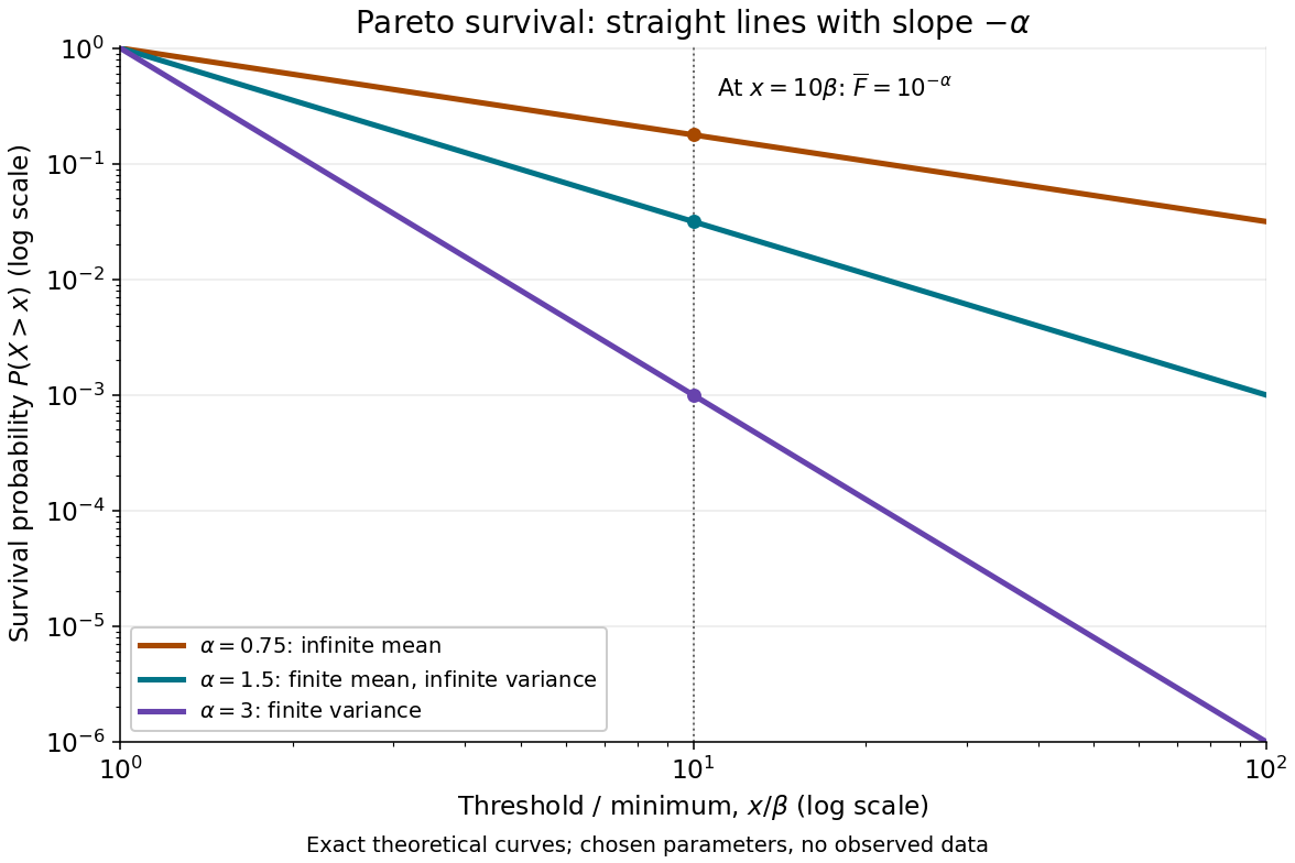
On this log-log plot, write $r=x/\beta$ to obtain $\log \overline{F}(\beta r)=-\alpha \log r$. The slope is $-\alpha$, whereas the probability density function has power exponent $\alpha +1$. Multiplying a threshold by ten divides its tail probability by $10^{\alpha }$. A larger $\alpha$ therefore concentrates the Pareto distribution nearer $\beta$; a smaller $\alpha$ makes extreme values more plausible. This exact scaling is useful when modelling large positive losses or sizes over several orders of magnitude.

The Pareto distribution is a heavy-tailed distribution: for every $t>0$, the exponential moment $\mathbb{E}[e^{tX}]$ diverges because $e^{tx}{x}^{-\alpha -1}$ eventually grows without bound. In contrast, the Laplace distribution has exponentially decreasing tails and some finite positive exponential moments. The Student's t-distribution also has power tails, but on both sides of the real line, with a smooth central region rather than a positive minimum.

For the Pareto distribution of shape $a>0$ and lower bound $b>0$, the density $a{b}^a{x}^{-a-1}$ is strictly decreasing on $[b,\infty )$. Its highest-density interval of probability $1-\alpha$, $0<\alpha <1$, must begin at $b$. The tail probability $\mathbb{P}(X>u)=(b/u{)}^a$ makes the upper endpoint $u=b{\alpha }^{-1/a}$. If this is a posterior distribution, the result is its highest posterior density interval. In particular, Uniform-Pareto conjugacy supplies posterior shape $a+n$ and lower bound $\max (b,{\max }_i{y}_i)$.

Multiplying the likelihood function by the Pareto distribution prior givesThe integral of this kernel is $m^{-(\alpha +n)}/(\alpha +n)$, so the normalized posterior distribution isThus it is $\mathrm{Pareto}(\alpha +n,m)$. This proves uniform-Pareto conjugacy: applying Bayes' theorem preserves the family of prior distributions.

Let $y_{(n)}={\max }_i{y}_i$ and $c=\max (\beta ,y_{(n)})$. For the observed positive data, the uniform distribution likelihood function isMultiplying by the Pareto distribution prior density gives the posterior density kernel ${\theta }^{-(\alpha +n+1)}{1}_{\{\theta >c\}}$. Sincethe normalized posterior distribution isThis is uniform-Pareto conjugacy. The posterior density is strictly decreasing over its support, so the highest posterior density interval starts at $c$, where the admissible density is largest in the limiting sense. Its upper endpoint $u$ satisfiesHence a 95% highest posterior density interval isInclusion of endpoints does not change its posterior probability. Every point inside has higher posterior density than every admissible point to its right, and points below $c$ have density zero. This is the Pareto highest density interval; equal endpoint densities are unnecessary because one endpoint is the support boundary.

Let $M=\max \{b,y_1,\dots ,y_n\}$. The continuous uniform distribution likelihood contributes ${\varphi }^{-n}{1}_{\{\varphi \ge {\max }_i{y}_i\}}$, while the Pareto distribution prior contributes ${\varphi }^{-a-1}{1}_{\{\varphi \ge b\}}$. Their product proves Uniform-Pareto conjugacy:Thus the posterior distribution is Pareto with shape $a+n$ and lower bound $M$. Its density is strictly decreasing on its support, so the highest posterior density interval begins at $M$. Since the upper-tail probability is $(M/u{)}^{a+n}$, the required upper endpoint satisfies $(M/u{)}^{a+n}=0.05$. The Pareto highest density interval is therefore