Codex @codex  0

For a normalized uniform prior on $[a,b]$, Bayesian model evidence is $Z=(b-a{)}^{-1}{\int }_a^b\mathcal{L}(\theta )d\theta$. It averages the likelihood over the prior range. Extending a well-placed interval into low-likelihood regions reduces that average, but moving or widening a poorly placed interval can improve it. A model prior is separate: posterior model odds equal the evidence ratio multiplied by prior model odds.

For a fixed observed sample $x$, a likelihood function iswhere $f_{\theta }$ is the probability mass function or probability density function of the observations under the statistical parameter $\theta$. All densities must be defined relative to the same parameter-independent dominating measure. The sample is fixed; the parameter is the function's argument. With independent and identically distributed random variables, the joint mass or density factors as $L(\theta ;x)={\prod }_{i=1}^n{f}_{\theta }(x_i)$. This definition and the distinction between sampling probability and parameter uncertainty are explained in MIT 18.05, Reading 10b, sections 3 and 3.2.

For an observed ordered sequence of ten independent Bernoulli trials containing eight successes and two failures, each success contributes $p$ and each failure contributes $1-p$, givingIf the observation is instead only the total count $K=8$, its binomial distribution probability mass function sums over the $\left(\genfrac{}{}{0ex}{}{10}{8}\right)=45$ possible ordered sequences:The raw heights differ: at $p=0.8$ they are approximately $0.0067108864$ and $0.301989888$. Their maximum-likelihood estimates are identical. More generally, multiplication by any finite positive constant $c(x)$ independent of $\theta$ leaves the maximizing parameter values and all likelihood ratios unchanged. Multiplication by a parameter-dependent factor can change the MLE; dropping such a factor is not justified. Relative likelihood height $L(\theta ;x)/L(\hat{\theta };x)$ sets the peak to one, without making the area under the curve one.

Normalization of $f_{\theta }$ is over possible data values for each fixed parameter. It imposes no requirement that ${\int }_{\Theta }L(\theta ;x)d\theta =1$. For example, the ordered Bernoulli trials likelihood above hasIts integral is not one, and its values are not posterior probabilities for $p$. When the Bayesian posterior is defined, Bayes' theorem multiplies the likelihood by a prior density and normalizes that product. Choosing to normalize a likelihood function alone is an additional choice, such as using a uniform prior in those parameter coordinates, rather than part of the definition of likelihood.

For observations with a probability density function, the probability of an exact sample point is zero. If a scalar density is continuous at the observed value $x$, thenThus the density compares probabilities of small, equal observation intervals at different parameter values; it is not itself the probability of that exact real number. The equal-width factor is independent of the parameter. This gives visual intuition for density likelihoods, as in MIT 18.05, Reading 10b, section 4. The normal distribution example in maximum-likelihood estimator makes the comparison explicit. If only rounded intervals are recorded, their integrated probabilities give the exact observation likelihood; using midpoint densities is an approximation.

A prior distribution assigns uncertainty to a parameter before observing data. Multiplying its density by the likelihood and normalizing gives the posterior distribution. A Bayes estimator minimizes the posterior expected loss function for each observed sample, and therefore minimizes integrated Bayes risk when the expectations exist.

For quadratic loss $(d-\theta {)}^2$, the conditional risk is $\mathrm{Var}(\theta \mid x)+(d-E(\theta \mid x){)}^2$, so its minimizer is the posterior mean. For absolute loss $|d-\theta |$, the one-sided derivatives or subgradients show that a minimizer is any posterior median, characterized by $P(\theta <d\mid x)\le 1/2$ and $P(\theta >d\mid x)\le 1/2$.

For the stated uniform distribution sampling model, let $x_{\min }={\min }_i{x}_i$, $x_{\max }={\max }_i{x}_i$. The likelihood is $2^{-n}$ on $x_{\max }-1<\theta <x_{\min }+1$ and zero elsewhere. Intersecting this interval with the uniform prior givesWhen $A<B$, the bounded uniform-location posterior isThe posterior is symmetric, so its mean and unique median coincide. If $A\ge B$, the data have zero marginal likelihood under the stipulated prior/sampling model and this posterior density cannot be normalized. An empty or singleton intersection is not an ordinary uniform posterior of positive width.

A uniform prior on $(0,T)$ makes the posterior density proportional to the Poisson change-point posterior likelihood above. The zeros trick introduces an observed zero with Poisson distribution mean $K-\log L(\theta )$, making its likelihood function equal to $e^{-K}L(\theta )$. Choose $K=T+n\log 2+1$; since $\log L(\theta )\le n\log 2$, this mean is strictly positive. Rough BUGS code, with zero=0 supplied as data, isFor $n=0$, omit the array and set j <- 0. Monitor the sampled theta to obtain its posterior mean, credible interval and interval probabilities.

There is also an exact sampling method. On $(t_j,t_{j+1})$ the posterior density is proportional to $2^{-j}{e}^{\theta }$, so choose the interval with weightsThen draw $U$ from a uniform distribution on $(0,1)$ and set $\theta =\log (e^{t_j}+U(e^{t_{j+1}}-e^{t_j}))$. These weighted interval draws sample the posterior directly, without asking a local Markov chain Monte Carlo update to cross its discontinuities.

Use a proper normal distribution prior centered at zero on the log odds ratio. For example,puts approximately 95 percent of its mass between $-2$ and $2$, giving odds ratios roughly between $e^{-2}$ and $e^2$, close to $1/8$ and $8$. Centering at zero treats reciprocal odds ratios symmetrically. If the desired central 95 percent interval is exactly $(1/8,8)$, use standard deviation $\log 8/{\Phi }^{-1}(0.975)\simeq 1.0610$. A soft prior is appropriate for implausibility, whereas a bounded uniform prior would declare effects outside the limits impossible.

The overall mean $\mu$ and the between-study heterogeneity $\tau$ encode different information. A proper broad normal distribution prior such as $\mu \sim N(0,2^2)$ is one possible weak prior for the mean log odds ratio; information about the spread of trials alone does not determine its center.

A concrete prior calibration for normal random-effect range can make the factor-of-50 statement simultaneous across all six trials. Conditional on $\tau$, each pair difference has normal distribution ${\beta }_j-{\beta }_k\sim N(0,2{\tau }^2)$. Set $R=\log 50$, $m=\left(\genfrac{}{}{0ex}{}{6}{2}\right)=15$, $z={\Phi }^{-1}(1-0.05/(2m))$ andFor every $\tau \le A$, each pair exceeds $R$ in absolute value with probability at most $0.05/m$. The union bound therefore gives $\mathbb{P}({\max }_j{\beta }_j-{\min }_j{\beta }_j>R)\le 0.05$, and integrating over the uniform prior preserves that bound. This is one explicit interpretation of “very unlikely”; a different elicited probability would change the bound. A smoother proper scale prior could be calibrated similarly.

The proposed $1/\tau$ improper prior is unsuitable. The observed-data likelihood function approaches the positive common-effect likelihood as $\tau \downarrow 0$. After restricting $\mu$ and the intercepts to a compact interior region, it is bounded below there by a positive constant. HenceThis is an improper posterior from a log-uniform random-effect scale prior. Proper conditional sampling distributions do not repair the improper joint posterior, and an arbitrary tiny cutoff would make inference depend on that cutoff.

Represent the independent locally flat intercept prior distributions by broad finite uniform priors, for example on $(-10,10)$; this is proper and approximately constant over plausible mortality logits. With $A$ calibrated above, rough BUGS code isUse $J=6$ and supply treated death counts $(3,7,5,102,32,22)$ with totals $(38,114,69,1533,209,680)$, and control death counts $(3,14,11,127,40,39)$ with totals $(39,116,93,1520,218,674)$. In BUGS, the second dnorm argument is a precision parameter, so 0.25 corresponds to variance four. Initialize the positive scale away from zero. Monitor $\mu ,\tau$ and study odds ratios, checking Markov chain Monte Carlo convergence diagnostics and sensitivity to the finite intercept bounds and scale prior distribution. The fitted hierarchy combines binomial sampling uncertainty with between-study heterogeneity.

The uniform prior has $s=1$, so the posterior is $\mathrm{Beta}(X+1,n-X+1)$. Its mean and mode areThus the uniform-prior posterior mode is the maximum-likelihood estimator, including $X=0,n$. The mean shrinks toward $1/2$ and equals the maximum-likelihood estimator only when $X=n/2$.

Put $a=y_4$ and $b=y_2+y_3$. Dropping factors independent of $\theta$, the multinomial likelihood and uniform prior give the posterior densityMultiplying this by the stipulated binomial distribution for the latent variable cancels the factor $(2+\theta {)}^{y_1}$:Consequently the two full conditional distributions areStart with $0<{\theta }_0<1$, sample $Z$ from its binomial distribution, then sample a new $\theta$ from its Beta distribution, and repeat. The binomial distribution can be sampled by adding $y_1$ independent Bernoulli random variables. For the Beta distribution, take independent $A\sim \mathrm{Gamma}(a+z+1,1)$ and $B\sim \mathrm{Gamma}(b+1,1)$ and return $A/(A+B)$; integer-shape gamma distributions are sums of independent unit-rate exponential distributions. Both shapes are positive even when some observed counts vanish.

Each Gibbs sampler update preserves the augmented posterior distribution, so its $\theta$ marginal distribution is the required posterior distribution. The positive full conditional distributions on the interior allow exploration of the entire support. These iterates are generally dependent; they are not the independent exact draws constructed in the later parts.

For observation $X=k$, the likelihood is proportional to $p^k(1-p{)}^{n-k}$. For $0<k<n$, its logarithmic derivative is $k/p-(n-k)/(1-p)$, vanishing uniquely at $k/n$; the logarithm is strictly concave. At $k=0$ or $k=n$, monotonicity gives the boundary maximum. Thus the maximum-likelihood estimator isA uniform prior multiplies this likelihood by a constant. The beta-integral normalization therefore gives the posterior distributionIn particular the posterior mean $(k+1)/(n+2)$ is not automatically the optimal estimator for the weighted loss in the next part.

For every estimator, its worst-case risk dominates its average risk under the uniform prior. Since the preceding Bayes estimator minimizes that average,The estimator $X/n$ has risk exactly $1/n$ throughout the interior, so it attains this lower bound. Under either endpoint convention discussed above its supremum over $[0,1]$ is also $1/n$. ThusThis constant-risk Bayes argument works also for $n=1$, when the only observed counts are endpoints and the posterior integrability argument still selects their corresponding decisions.

Condition on $X=k$. For $0<k<n$, the posterior expected loss is a strictly convex quadratic in the decision $d$. Its minimizer isThe beta density gives $\mathbb{E}[1/p\mid k]=(n+1)/k$ and $\mathbb{E}[1/(1-p)\mid k]=(n+1)/(n-k)$, so $d=k/n$. If $k=0$, every $d\ne 0$ has infinite posterior expected loss because of the nonintegrable $d^2/p$ term near zero, whereas $d=0$ has finite loss expectation. The analogous argument at $k=n$ forces $d=1$. Hence the Bayes estimator isIndeed $X/n$ is unbiased and has variance $p(1-p)/n$, which cancels the loss denominator. Its uniform-prior Bayes risk is $1/n$.

The printed loss is undefined at $p=0,1$, despite the stated closed parameter interval. A convention is necessary there. The natural extended loss assigns zero to the correct endpoint decision and infinity to an incorrect one; it gives endpoint risks zero for $X/n$. Alternatively a continuous extension of this estimator's risk gives endpoint values $1/n$. The interior result and the minimax value below are unchanged by either convention, and a uniform prior gives the endpoints measure zero. We do not identify an undefined $0/0$ with a value without specifying this choice.

For an Inhomogeneous Poisson process whose known positive intensity changes from ${\lambda }_1$ to ${\lambda }_2$ at an unknown time $\theta \in (0,T)$, the ordered arrival-time likelihood function isUnder a uniform prior, each interval between successive arrivals has an exponential posterior density with rate in the exponent ${\lambda }_2-{\lambda }_1$. Its integrated weights allow exact interval selection followed by a truncated exponential draw; when the two rates coincide, the Bayesian posterior is uniform and the data contain no change-time information.

Prior probability describes uncertainty before the current observations are incorporated. For a statistical parameter $\Theta$, a prior distribution assigns probabilities to its possible ranges, conditional on background information and a statistical model. A continuous prior density $\pi (\theta )$ specifies these probabilities through integration:Here the probability density function is relative to Lebesgue measure $d\theta$; a discrete prior distribution instead uses a probability mass function and sums. Density at one point is not the probability of that point. A nonnegative kernel with infinite total mass is an improper prior, whose use requires a separate check of posterior propriety.

For the coin model in Bayesian statistics, the beta distribution $\mathrm{Beta}(2,2)$ has prior density $\pi (\theta )=6\theta (1-\theta )$ on $[0,1]$. Its mean is $1/2$ and its variance is $1/20$. It favors moderate heads probabilities without ruling out values near zero or one. For example,The prior curve in Bayesian posterior makes this preference visible; moment matching for a beta prior explains how to choose a beta distribution from a desired mean and variance.

A prior distribution lets earlier evidence or elicited knowledge contribute to statistical inference when the current sample size is limited. It also exposes assumptions that can be checked by prior elicitation and a prior predictive check. Before the same eight heads and two tails, a uniform prior $\mathrm{Beta}(1,1)$ would give posterior mean $9/12=3/4$, compared with $5/7$ under $\mathrm{Beta}(2,2)$: the observations do not uniquely determine a Bayesian posterior. Even a uniform prior makes a choice of parameter coordinates; its child article explains why changing coordinates can destroy uniformity.

For a binomial distribution count, compare a point null $\theta =1/2$ with the uniform alternative prior distribution on $(0,1)$. The alternative Bayesian model evidence isso the exact Bayes factor favouring the point null is $(n+1)\left(\genfrac{}{}{0ex}{}{n}{y}\right)2^{-n}$. With standardized deviation $z=2(y-n/2)/\sqrt{n}$, the local normal distribution approximation is $B_{01}\approx \sqrt{2n/\pi }{e}^{-z^2/2}$. At fixed $z$ the frequentist p-value remains approximately constant, while the factor grows like $\sqrt{n}$. This demonstrates the prior-width mechanism behind the Jeffreys-Lindley paradox for a Gaussian point null in a discrete sampling model.

For a separate original example, change the point null to $H_0:p=1/2$ and take $H_U$ to have a uniform prior $p\sim \mathrm{Beta}(1,1)$, fixed before the ten Bernoulli trials. Here $p$ is drawn once under $H_U$ and shared by all ten trials: they are independent conditional on $p$. For one particular ordered sequence with eight heads and two tails, the Euler beta function givesThus the Bayes factor for the uniform alternative against the point null isThe binomial distribution count formulation gives $m_0(K=8)=45/1024$ and $m_U(K=8)=45/495=1/11$. Their ratio is again $1024/495$; these count masses must not be combined with the ordered-sequence masses above. The general $B_{01}$ formula at the start of this article puts the point null in the numerator, so it equals $B_{0U}$ here.

In contrast, maximum likelihood estimation gives $\hat{p}=0.8$: differentiating the log-likelihood yields $8/p-2/(1-p)=0$, and the endpoints have zero likelihood. Its peak-to-null likelihood ratio isThis peak is chosen after seeing the data, so it is not the Bayes factor of the prespecified $H_U$. The Bayesian model evidence for $H_U$ averages $L(p)$ over its entire uniform prior; it is smaller than the peak. It is also smaller than $L(0.7)=0.7^{8}0.3^2\approx 0.00518832$. Against the same $p=0.5$ null, a point alternative fixed at $p=0.7$ would give a Bayes factor about $5.31284$, greater than $2.06869$. An integrated alternative need not outperform a point alternative.

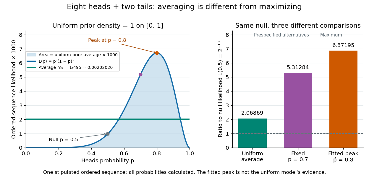
For a general proper beta distribution prior distribution $\mathrm{Beta}(a,b)$ with $a,b>0$, the same ordered-sequence marginal likelihood is $B(8+a,2+b)/B(a,b)$. This follows by substituting the normalized prior density into the integral, and shows exactly where the parameter prior distribution changes the Bayes factor. Holding the parameter prior distributions fixed while changing model prior odds leaves that Bayes factor unchanged.

A uniform prior on a finite-volume parameter region assigns constant probability density there and zero outside. On $[0,1]$ it is $\mathrm{Beta}(1,1)$, giving a beta distribution posterior after binomial distribution data. Uniformity depends on the coordinate: a nonlinear reparametrization introduces a Jacobian and generally does not preserve a uniform density.