Topics (384k) Articles (398k) Users (410) Discussions (242) Comments (383) Files (13k) New article

A noise-whitened pressure sensing matrix measures how a contact pressure pattern changes sensor outputs relative to their joint noise, rather than their raw numerical size. For a linear measurement modelassume the error covariance is positive definite. Choose an invertible matrix satisfying . ThenThe transformed errors have identity covariance. This is the whitening transformation documented in the primary SciPy covariance interface; its example obtains approximately identity sample covariance from simulated observations.[ref]
A Cholesky decomposition supplies . Compute and by solving triangular systems rather than forming an inverse unnecessarily. The least-squares residual becomesThus an output change is significant according to its noise covariance, not merely the Euclidean length of the raw readings. The original pressure basis and its units must still be stated; whitening rows does not remove arbitrary column rescalings.
For an original two-channel example, use numerical pressure values in kilopascals andThe separate standard deviations are and with correlation . A residual whitens to , giving squared length about . The residual instead whitens to , giving squared length . Treating the channels as independent would assign both residuals squared standardized length two. The positively correlated noise makes opposite-sign discrepancies much less plausible than a shared shift.
A simple repeated-measurement model illustrates the information consequence. If two sensors measure the same scalar pressure with equal standard deviation and correlation , their mean has variance . At the standard deviation is about , rather than the independent-channel value . Adding an almost duplicate channel therefore supplies little improvement for that common pressure.
The pressure-map information matrix is . In a full-column-rank linear Gaussian model with known , the unconstrained weighted least-squares estimate has covariance . Small singular values of identify near-null directions of a pressure sensor array after accounting for noise. Alternative whiteners differ by an orthogonal row transformation and give the same information matrix; an individual whitened row need not represent one physical sensing cell.
A proposed array characterization applies repeatable known pressure patterns, estimates the channel covariance from repeated residuals, and checks the covariance on independent repeats after whitening. Drift and response-model uncertainty must be included if they belong to the intended error model. If is singular, a simple inverse whitening is unavailable: exact zero-noise constraints and redundant stochastic directions need separate treatment. A visually smooth pressure reconstruction does not establish that its weak directions were measured precisely.
The microplate footprint is the base outline used to locate a microplate in a carrier, gripper or microplate reader. It defines a mechanical interface rather than the liquid volume or the detailed geometry of individual wells. A common nominal rectangle promotes compatibility, but its dimensional tolerances and measurement locations must accompany the nominal values.
The primary footprint standard gives length127.76mm and width85.48mm. Within12.7mm of the outside corners, its specified tolerances are ; measured anywhere along the sides, they are . Its default dimensional reference temperature is .[ref]
Microplates - Footprint Dimensions by SLAS. §1.2 and §4.1.1.1–4.1.1.2, reference conditions and measurement locations
Using the tighter near-corner tolerance for every location would misread the specification.For an original rectangular-envelope calculation, take a carrier opening128.40mm long and86.10mm wide. The standard's full-side upper limits are128.26mm and85.98mm, leaving total length and width clearances0.14mm and0.12mm. If the plate and opening are centered in this simplified model, those become0.07mm and0.06mm per side. Designing only from nominal dimensions would instead suggest much larger total clearances0.64mm and0.62mm.
The calculation concerns the stated planar envelope. Corner shape, flange geometry, vertical clearance, positioning features and the carrier's own tolerances can also determine whether a real plate seats correctly. The footprint standard separately specifies a continuous base outline and corner-radius requirements, rather than reducing the entire interface to two nominal lengths.[ref]
A footprint check can use calibrated dimensional measurements at the specified locations and conditions. It should distinguish a length measurement from a functional fit test: a plate that enters one carrier does not by that observation alone establish every standard dimension, and agreement in two measured dimensions does not establish optical suitability. Well-bottom transmission and microplate path-length correction remain separate parts of the optical measurement chain.
The standard's foreword identifies dimensional variation between suppliers as an automation problem. This supplies the practical motivation for the interface: a plate should arrive at a predictable physical location so that downstream handling and measurements can be repeatable.[ref]
Microplates - Footprint Dimensions by SLAS. Foreword, dimensional variation and automated-instrument compatibility
Uncertain variance in heterodyne lognormal bias correction matters when a measured overlap is corrected using an estimated, rather than known, logarithmic variance. The known-variance correction is a nonlinear function of that estimate, so replacing the variance by an unbiased estimate does not automatically preserve unbiasedness of the corrected overlap.
Suppose , with , and use . If the variance estimate is independent of the overlap readout,Even if , Jensen's inequality gives . Consequently the mean corrected estimate is at least under these independence and unbiased-variance assumptions. Equality requires a nonrandom variance estimate in the ordinary finite-variance case.
An original exact example uses a variance estimate from an independent normal calibration sample, with following a chi-squared distribution with degrees of freedom. Its Laplace transform givesThe logarithm of this factor is , which is positive for . With stipulated and , the factor is : about a 9.91% remaining mean shift. This intentionally broad statistical example is not a typical receiver specification.
For fixed and large , the logarithm is . More independent calibration information reduces this effect. Merely taking more overlap readings while retaining the same uncertain variance estimate does not remove its influence.
Dependent variance correction in heterodyne normalization requires the joint quantity instead of the product of expectations above. A variance inferred from the same readout cannot simply be declared independent. Propagate the joint calibration and readout model, with a stated target summary. JCGM 101 treats input distributions from prior uncertainty calculations and numerical propagation explicitly.[ref]
The optical gain-matching condition for heterodyne normalization still concerns physical calibration paths. This calculation addresses the statistical correction of residual log-errors; it does not imply that an imperfect RF or DC calibration can be repaired solely by subtracting a fitted variance.
The Komodo dragon, Varanus komodoensis, is a large predatory lizard native to Indonesian islands. It takes animal prey and also scavenges. The scientific name identifies the species, while the familiar name does not denote a separate evolutionary group from other lizards.[ref]
Its reproduction provides a striking example of facultative parthenogenesis: production of offspring without fertilization can occur in a species that also reproduces sexually. A 2006 study examined offspring from two females isolated from males at separate institutions. Microsatellite genotypes and reproductive histories supported maternal-only inheritance; one female later also produced sexually conceived offspring.[ref]
Parthenogenesis in Komodo dragons by Phillip C. Watts and others. Abstract and supplementary genotyping/reproductive histories
Genetic comparison matters because the absence of a male at laying does not alone exclude earlier mating or stored sperm. As a simplified example, a mother carrying alleles and at a locus might produce a parthenogenetic offspring carrying two copies of . That offspring contains only a maternal allele but is not an identical genetic copy of its mother. Evidence from several loci is more informative than this single-locus illustration.
The observation therefore distinguishes parthenogenesis from simple cloning and shows that reproductive mode can vary within a species. It does not establish that all isolated females must reproduce this way or that every form of animal parthenogenesis has the same genetic mechanism.
Squamata is the reptile lineage containing lizards, snakes and amphisbaenians. It belongs within lepidosaurs, whose other living branch is represented by the tuatara. Snakes are nested among lineages commonly called lizards, so excluding snakes does not leave a complete evolutionary branch.
The relationships require evidence beyond superficial similarity: elongated, limbless bodies can arise in different lineages. A 2015 analysis combined hundreds of anatomical characters with dozens of genes from living and fossil groups to compare competing arrangements.[ref]
Integrated Analyses Resolve Conflicts over Squamate Reptile Phylogeny and Reveal Unexpected Placements for Fossil Taxa by Tod W. Reeder and others. Abstract: integrated morphology and molecular data
This makes Squamata a useful example of how phylogenetics tests anatomical interpretations against molecular evidence while retaining fossils that have no recoverable sequence data.A Kähler-Einstein metric is a Kähler metric whose Ricci tensor satisfiesfor a real constant . Equivalently, its Ricci form satisfies , where is the Kähler form. It combines the compatibility of complex and Riemannian geometry with an Einstein curvature condition.
In holomorphic coordinates, take . The Ricci form is . A constant positive Hermitian matrix therefore gives : the flat metric on , and its quotient by a full lattice, are Ricci-flat examples. The Fubini-Study metric on Complex projective space gives a positive- example, with the numerical value depending on the metric normalization.
The equation is a nonlinear condition on a local Kähler potential, through the logarithmic determinant of its complex Hessian. This is why complex Monge-Ampère equations enter existence questions. Not every Kähler metric satisfies the Einstein condition.[ref]
Lectures on Kähler Geometry by Andrei Moroianu. Sections 11 and 13, Ricci form and Kähler-Einstein condition
Relative calibration error in an isotope-corrected stiffness ratio is the fractional error remaining when spectral calibration affects the two compared bands differently. Write the model of isotope-corrected Raman stiffness ratio as , where and the positive denote vibrational wavenumbers. For small errors,The mass correction does not remove differential spectral calibration error.
A useful calibration model is , with common and separate gain errors and offsets . Its spectral contribution becomeswith the mass term added if uncertain. A single multiplicative scale cancels exactly when no additive error is present. Separate gains do not: comparing two spectra calibrated independently can lose that cancellation.
For an original example, take and . A differential gain creates about relative error in . A common offset instead contributes about . If the separate gains each have independent standard uncertainty, their combined contribution to the relative standard uncertainty of is .
The separate spectral-calibration gains in isotope stiffness inference must therefore be distinguished from a shared reference error. Covariance propagation keeps precisely those shared and separate influences.[ref] Recording both samples with the same validated spectral scale can help, but drift or changed dispersion can still produce differential errors.
The primary graphene isotope experiment measured Raman bands over isotope concentrations and laser excitation energies and found the harmonic-oscillator mass dependence.[ref]
Probing carbon isotope effects on the Raman spectra of graphene with different ¹³C concentrations by Bruno R. Carvalho and others. Abstract, isotope-mass dependence of Raman frequencies
Small residual stiffness changes require the additional calibration and mode-model checks above; the numerical errors here are chosen examples, not quoted experimental uncertainties.An equitable partition of a finite graph groups vertices so that any two vertices in one cell have the same number of neighbours in each cell. For a simple graph with cells , this means that numbersdo not depend on which in is selected. Here denotes the set of neighbours of . These counts form the equitable quotient matrix . An equitable partition need not be a proper vertex colouring and need not have cells of equal sizes.[ref]
Practical graph isomorphism, II by Brendan D. McKay and Adolfo Piperno. Section3.1 and footnote1, equitable-partition terminology
An original five-vertex path graph has an equitable partitionEach endpoint has one neighbour in ; each member of has one neighbour in and one in ; the middle vertex has two neighbours in . Although the graph is undirected, is not symmetric matrix, because its entries count neighbours per vertex rather than total edges between cells. Counting those edges from both ends gives .
The counts also compress an exact part of the adjacency matrix. Let be that matrix and let have one column per cell, with for and zero otherwise. ThenIndeed, counts neighbours of in , which is exactly . Hence implies . Since nonempty disjoint cells make the columns of linearly independent, gives : every eigenvalue of is an eigenvalue of . For the displayed example, these include and .
An equitable partition preserves neighbour counts, not all adjacency information. The disjoint union of graphs of a triangle and a four-vertex cycle has an equitable one-cell partition, since every vertex has two neighbours. Nevertheless, no graph automorphism can send a triangle vertex to a four-cycle vertex: their connected components of a graph are not isomorphic. This distinguishes equitable cells from symmetry orbits and explains why colour refinement may leave ambiguity.
Colour refinement repeatedly separates vertices of a graph according to the colours of their neighbours. Its colours are labels for classes of vertices with the same currently visible structure; they are not a proper vertex colouring requiring adjacent vertices to differ. In individualization-refinement graph search, colour refinement reduces ambiguity before the algorithm branches.[ref]
Practical graph isomorphism, II by Brendan D. McKay and Adolfo Piperno. Section3.1, equitable refinement and Algorithm1
Let be a vertex's colour after round . One conceptual update assigns a common new colour exactly when both the previous colour and neighbour-colour multiset agree:The encoding must give distinct labels to distinct signatures. Retaining prevents old classes from merging. When no class splits, the resulting partition of a set is an equitable partition: vertices in the same cell have equal numbers of neighbours in every cell.
For an original example, start all vertices of the six-vertex path graph with the same colour. The first round separates endpoints from internal vertices . The next separates , which each have an endpoint neighbour, from , which do not. The three cellsare then stable. Reflection of the path exchanges the two vertices in each cell, so the remaining pairs are compatible with a genuine graph automorphism.
Colour refinement is invariant under vertex relabeling. To compare two graphs, colour signatures must be encoded consistently across both, for example by refining their disjoint union of graphs with shared initial colour meanings. A different count of vertices in a resulting colour class certifies graph non-isomorphism.
Agreement is weaker than isomorphism. Starting with one colour, both the complete bipartite graph and the triangular prism graph remain one six-vertex cell because every vertex has three neighbours. Yet the prism has triangles and has none. This failure motivates individualizing vertices and searching further; stable colour classes are not, in general, proof that all their vertices are related by graph automorphisms.
An electronic comparator registers a pulse only if its input reaches the chosen threshold. For an initially uncharged capacitor driven through an electrical resistance , a short rectangular pulse may end before that happens. The resulting threshold-crossing time of a finite rectangular pulse through an RC load depends on threshold and pulse duration, as well as the time constant ; it is not determined by group delay alone.
Take a positive input electric potential difference for , zero input outside that interval, and output across a capacitance . Include the source's effective series electrical resistance in . The initial condition is . Kirchhoff's voltage law and the capacitor current relation give the first-order linear differential equationThe output is a continuous function and reaches its maximum at the pulse's falling edge:The input jumps there, but an ideal capacitor's stored electric charge cannot change discontinuously under the finite currents of this model.
Choose a fixed threshold with . Solving the rising exponential function using a natural logarithm givesIf , the output never reaches the threshold. At , it touches the threshold only at its peak; the ideal time spent strictly above threshold is zero. A nonzero high interval in an ideal non-inverting electronic comparator requires . This is RC pulse-width discrimination: different input durations can give a missing pulse or a finite output pulse even when their input heights are equal.
For , solving the falling exponential decay givesHere is the time above threshold for an RC-filtered rectangular pulse, before any electronic comparator switching dynamics. It is not generally the input duration . Just above , differentiation gives and hence to first order; a half-height threshold gives slope two at the detection boundary.
For an original numerical example, take , , , and , so . A input peaks at only and is rejected. A input peaks at and givesThese are model calculations, not recorded instrument traces.
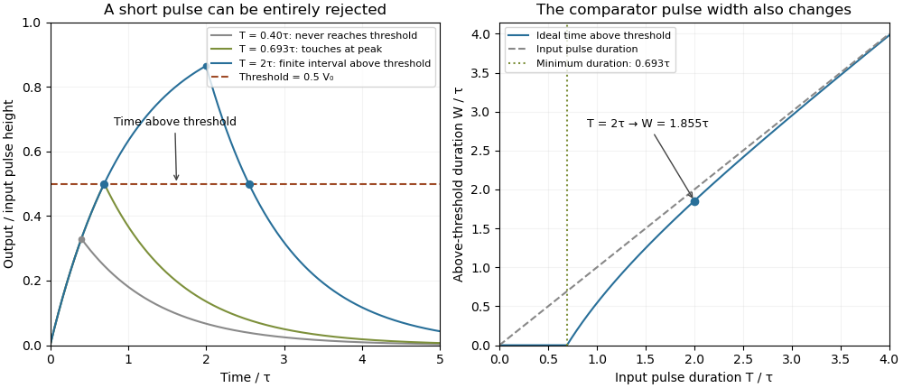
A threshold near the asymptotic input height is also especially sensitive to noise and threshold measurement uncertainty. Holding the absolute input height and fixed, the threshold timing sensitivity of an RC step response isFor the same , model, a effective threshold perturbation gives approximately of timing change at , but at , by first-order uncertainty propagation. The rectangular pulse must still last long enough to reach the selected threshold; changing together with is a different sensitivity calculation.
A bench test uses a pulse generator and an oscilloscope to record both the applied electric potential difference and the capacitor output. Sweep while keeping and the actual threshold fixed, and allow enough time between pulses for the measured initial output to be negligible at the desired precision. Include probe and comparator-input capacitance in . MIT's laboratory measures RC decay with a capacitor, a resistor and square-wave excitation; that gives a directly measurable component-value time constant.[ref]
Laboratory 11: Sinusoidal Steady State Response of RC and RL Circuits by MIT OpenCourseWare. Printed pp. 1–2, component values and decay/phase measurements
The pulse-duration sweep proposed here extends that decay measurement to a threshold observation. A real electronic comparator's input offset voltage, hysteresis and finite switching time must be separated from the ideal RC crossing times; a Schmitt trigger uses different rising and falling thresholds.A gear tooth engagement threshold is the relative approach or total load at which a previously separated tooth pair starts carrying compressive contact force in a stated model. Geometric overlap from the gear contact ratio does not guarantee that every potentially overlapping pair already carries load. Gaps, errors and deformation affect the gear mesh active-contact set.
For an original unilateral linear-spring model, writewith , common approach and initial gap . Pair begins to carry load as rises above . The corresponding total-load threshold isThis threshold includes the forces already carried by earlier contacts. It is not generally obtained by multiplying pair 's own stiffness by its gap.
Take , , and . The second pair begins at total load . At , approach is and the second pair remains unloaded. At ,gives , forces and , and gear tooth load fractions and .
At the ideal threshold itself, the new contact contributes zero force but changes the one-sided gear mesh tangent stiffness. The force is continuous while its slope can jump. Finite contact geometry and nonlinear local Hertzian contact can smooth or alter this elementary linear-spring picture.
A controlled quasistatic test can increase total mesh load at approximately fixed contact position while measuring relative displacement and individual tooth-root strain. A change in response slope suggests a contact transition, but support motion and measurement resolution must be considered before assigning it uniquely to a tooth pair. Primary dynamic gear analysis couples tooth stiffness and calculated loads as contact position changes, underscoring that engagement cannot be inferred from tooth count alone.[ref]
The gear mesh tangent stiffness is the local derivative of total mesh force with respect to a specified relative approach, with contact position and other state variables held fixed:It predicts a sufficiently small incremental force . Unlike a reference-based secant stiffness , it describes the local response rather than the whole loading interval.
For away from any gear tooth engagement threshold,Only members of the gear mesh active-contact set contribute. With , and gaps and , the gear mesh tangent stiffness is before the second contact and after it. At approach , an additional gives more force within the same branch.
The ideal transition at has distinct left and right derivatives. A centered finite difference with any sufficiently small positive giveswhere numerical displacements are expressed in micrometres. The value is the mean of the two branch slopes; it does not establish a unique derivative at the corner, even as shrinks.
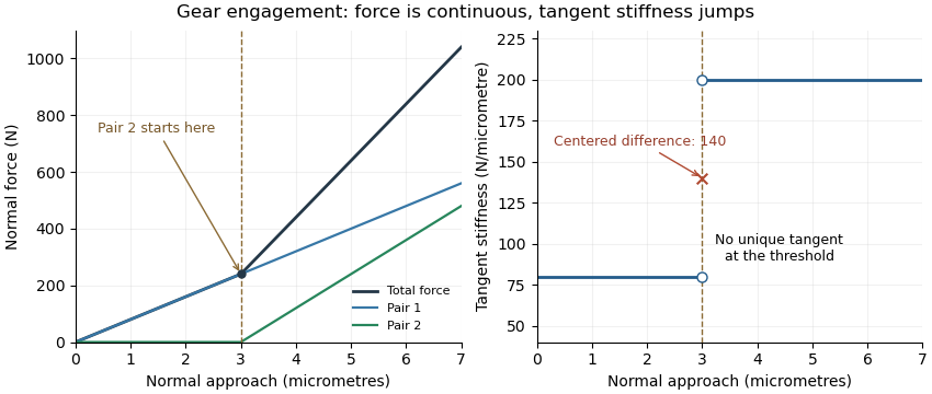
Original unilateral-contact model: continuous force, a gear tooth engagement threshold, and distinct one-sided gear mesh tangent stiffness values
. Details. The measured displacement channel also matters. If a contact stiffness is in series with support stiffness , their mechanical compliances add, givingA measurement spanning the whole assembly would therefore not isolate the contact stiffness.
For a perturbation experiment, report the mean load, mesh position, displacement endpoints and whether the increment crosses a contact transition. A primary NASA analysis used a coupled tooth-stiffness/dynamic-load calculation; the derivative above explains a local quasistatic limit, rather than replacing that dynamical model.[ref]
An unresolved Gaussian pulse-width estimate occurs when the measured correlation width and characterized response do not establish a positive pulse width with useful precision under the assumed Gaussian model. It is a limitation of the measurement and inference, not evidence that the pulse has zero duration.
In Gaussian pulse-width deconvolution uncertainty, the inferred full width at half maximum isFor , a positive central value exists. Whether the data resolve it depends on the uncertainty in , the response model and their covariance, not just on the sign of the central radicand.
Take original central values and . They give and . Independent standard uncertainties give, to first order,This uncertainty is almost three times the central difference. Propagating once more through the square root gives ; that symmetric approximation is poorly suited to the boundary . The GUM requires attention to higher-order terms when nonlinearity invalidates the first-order approximation.[ref]
Guide to the expression of uncertainty in measurement by JCGM. §5.1.2, nonlinear functions and higher-order terms; §5.2, covariance
A simple range calculation makes the difficulty visible without assigning a probability. Suppose only that plausible widths lie in and . These ranges include equal widths, hence , while their maximum positive radicand is , giving . These stipulated ranges are not a calibrated confidence interval; they demonstrate sensitivity to response uncertainty.
A negative observed need not imply an imaginary physical duration: noise, incorrect response characterization or a non-Gaussian pulse can invalidate the naive inversion. Conversely, dropping all negative simulated radicands and averaging the rest conditions on a selected subset and biases the inference. A Monte Carlo method must implement a stated input or likelihood model and a justified treatment of the physical boundary.
Report the measured and response widths, their conventions, uncertainties and dependence. An upper limit is meaningful only with its statistical construction and coverage assumptions. Improved response characterization or an independent temporal measurement can resolve the ambiguity; quoting more digits of the positive square root cannot.
A heterodyne RF-to-DC gain transfer check tests whether the calibration converting a beat-frequency measurement into current amplitude is compatible with the calibration of the separate arm currents. The gain-matching condition for heterodyne normalization involves amplitude gains, so an RF power gain cannot be substituted without conversion.
For corrected peak beat current and arm currents , the normalized overlap is . Suppose an electrical model gives sinusoidal peak current through a known resistive load . Its average beat power isSource/load division and impedance corrections must already be included when relating that load current to the detector-current convention. A factor converting power is therefore square-rooted when converting amplitude.
Let measured RF power carry multiplicative factor , while the arm currents carry factors . Under this model,Cancellation requires . With one common DC current factor , the condition is , not .
An original example takes . An RF power factor 1.21 produces amplitude factor 1.10 and cancels in the normalized overlap. Applying RF power factor 1.10 instead leaves multiplier , despite using the same numerical gain label in both paths. The example isolates heterodyne amplitude-versus-power gain conversion, rather than a change of optical overlap.
NIST's receiver experiment measured microwave power and separately corrected sensor calibration, electrical loss and impedance matching. Its two-laser optical source used polarization and spatial matching to establish calculable modulation.[ref]
Frequency response metrology for high-speed optical receivers by Paul D. Hale and others. PDF pp. 1–2, Heterodyne measurements and Eqs. 1–4
Those separate operations make the RF-to-DC comparison a physical calibration problem.Record peak versus RMS conventions, frequency response, load model and arm-current calibration. Test a known or independently characterized modulation while varying power within the linear range. Changed polarization, aperture clipping or optical alignment can alter the true overlap and imitate a gain-transfer defect, so one unexplained normalized ratio does not uniquely diagnose the electrical path.
A floating-pinion robust contact margin is the smallest two-contact compression margin allowed by a stated set of uncertain parameters. It strengthens a nominal floating-pinion compression margin by checking every admissible parameter combination, while retaining the assumptions of the underlying contact model.
Let be the common approach and the equilibrium imbalance in the symmetric linear model. If the admissible pairs form a set , defineFor displacement from equilibrium with , the smaller contact compression is at least . Thus guarantees positive compression for both contacts throughout the bounded motion. Equality permits zero compression and does not guarantee maintained compressive contact.
For independent interval bounds, or a bounding rectangle containing all possible pairs,This is exact when every pair in the rectangle is admissible. If the rectangle includes impossible combinations, it remains a conservative lower bound on .
A correlated floating-pinion uncertainty set can materially change the conclusion. In an original example, all quantities are in micrometres andHere stays positive, so for every allowed . The exact joint-set margin is . Treating the ranges independently instead gives . An amplitude passes the joint-set guarantee with residual compression , but fails the rectangular sufficient test. Failure of a conservative test does not itself demonstrate contact loss.
The admissible set must come from defensible parameter bounds, including any shared mounting or thermal effects. A covariance estimate alone supplies no absolute bound for all realizations. If the motion amplitude also depends on uncertain parameters, a direct bound on can preserve correlations that separate worst-case bounds discard.
Floating mounting was physically motivated by face-gear load sharing. NASA's primary report describes mounting freedom and slow-roll torque-division tests; those observations motivate the contact model, but do not validate every dynamic or uncertainty assumption above.[ref]
Development of Face Gear Technology for Industrial and Aerospace Power Transmission by Gregory F. Heath and others. Introduction, printed pp. 1–2; Conclusions, printed p. 84
Once a contact opens, a floating-pinion contact-loss check must use the appropriate changed force law.Rank deficiency from deterministic spectral upsampling occurs because a deterministic map cannot manufacture independent measurements. For and input covariance matrix ,When the output has more channels than the input, its covariance matrix is necessarily singular. Covariance of count-conserving rebinned Raman channels gives the conserved-count example and its full propagated uncertainty.[ref]
Using that parent's two-to-three channel map, the output always satisfies . If the input readings are and , the rebinned vector is . Recovering the original readings as and shows that the third displayed number is not a third independent observation.
For an original fitting example, suppose both input means equal an unknown and their independent measurement-error variances are known to be . Fitting in the original channels gives , with variance . A correct generalized least squares fit after rebinning gives the same result and uncertainty. It must use the singular covariance on its supported range, for example through the Moore-Penrose inverse, together with the exact linear constraints.
The range restriction in singular-covariance spectral fitting matters if a proposed output model fails those constraints. A residual along cannot arise from this rebinning model at all. Merely inserting a pseudoinverse into a quadratic objective would assign zero penalty to that impossible direction. Either enforce the range condition or supply a physically justified additional noise model; adding a small diagonal term solely to make the matrix invertible changes the statistical assumptions.
The motivating Raman apparatus measures detector-array spectra before any subsequent numerical grid change.[ref]
Femtosecond Broadband Stimulated Raman: A New Approach for High-Performance Vibrational Spectroscopy by David W. McCamant and others. Instrumentation, array detection and spectral calibration; Data Collection, equation 4
Working on the original grid often avoids this singular fitting problem while retaining the actual measurement information.The effective convolution kernel size is the bounding extent of a dilated convolution kernel along a spatial axis. For sampled coefficients with convolution dilation , their offsets are . The first-to-last displacement is , so including the first position givesThis extent determines the kernel footprint used in spatial shape calculations; it is not generally the number of coefficients.[ref]
For a two-dimensional example, choose a sampled kernel shape with dilation . Its row offsets are and column offsets are . The bounding shape is thereforeThere are six sampled spatial positions inside a twenty-position bounding box. Fourteen intermediate positions are absent from the sampling pattern.
With three input neural network channels and four output channels, ordinary dense channel connectivity usesweights and optionally four biases, giving parameters. A general dense five-by-four kernel with the same channel counts would have weights. Representing the dilated operation that way would require of them to be fixed zeros, rather than independently learned parameters.[ref]
For an unpadded -by- input and convolution stride one, the output grid isMore generally, for one axis with symmetric zero padding and stride ,when the padded input accommodates the footprint. The floor function counts admissible filter origins.[ref]
The effective size is a geometric quantity for one layer. The complete neural network receptive field through several layers additionally depends on their kernels, strides and connections. Likewise, changing stride moves the spacing of origins; changing dilation changes the footprint at each origin. Keeping bounding extent, sampled-position count and learned-parameter count separate avoids confusing three different sizes.
Pinned article: Introduction to the OurBigBook Project
Welcome to the OurBigBook Project! Our goal is to create the perfect publishing platform for STEM subjects, and get university-level students to write the best free STEM tutorials ever.
Everyone is welcome to create an account and play with the site: ourbigbook.com/go/register. We belive that students themselves can write amazing tutorials, but teachers are welcome too. You can write about anything you want, it doesn't have to be STEM or even educational. Silly test content is very welcome and you won't be penalized in any way. Just keep it legal!
Intro to OurBigBook
. Source. We have two killer features:
- topics: topics group articles by different users with the same title, e.g. here is the topic for the "Fundamental Theorem of Calculus" ourbigbook.com/go/topic/fundamental-theorem-of-calculusArticles of different users are sorted by upvote within each article page. This feature is a bit like:
- a Wikipedia where each user can have their own version of each article
- a Q&A website like Stack Overflow, where multiple people can give their views on a given topic, and the best ones are sorted by upvote. Except you don't need to wait for someone to ask first, and any topic goes, no matter how narrow or broad
This feature makes it possible for readers to find better explanations of any topic created by other writers. And it allows writers to create an explanation in a place that readers might actually find it.
Figure 1. Screenshot of the "Derivative" topic page. View it live at: ourbigbook.com/go/topic/derivativeVideo 2. OurBigBook Web topics demo. Source. - local editing: you can store all your personal knowledge base content locally in a plaintext markup format that can be edited locally and published either:This way you can be sure that even if OurBigBook.com were to go down one day (which we have no plans to do as it is quite cheap to host!), your content will still be perfectly readable as a static site.
- to OurBigBook.com to get awesome multi-user features like topics and likes
- as HTML files to a static website, which you can host yourself for free on many external providers like GitHub Pages, and remain in full control

Figure 2. You can publish local OurBigBook lightweight markup files to either OurBigBook.com or as a static website.
Figure 3. Visual Studio Code extension installation.
Figure 5. . You can also edit articles on the Web editor without installing anything locally. Video 3. Edit locally and publish demo. Source. This shows editing OurBigBook Markup and publishing it using the Visual Studio Code extension. 
- Infinitely deep tables of contents:




All our software is open source and hosted at: github.com/ourbigbook/ourbigbook
Further documentation can be found at: docs.ourbigbook.com
Feel free to reach our to us for any help or suggestions: docs.ourbigbook.com/#contact