Topics (349k) Articles (361k) Users (423) Discussions (237) Comments (383) Files (12k) New article

A mass spectrum displays detected signal against mass-to-charge ratio. Peak positions identify candidate ions; peak areas give isotopic abundances only after the response and overlapping contributions have been accounted for.
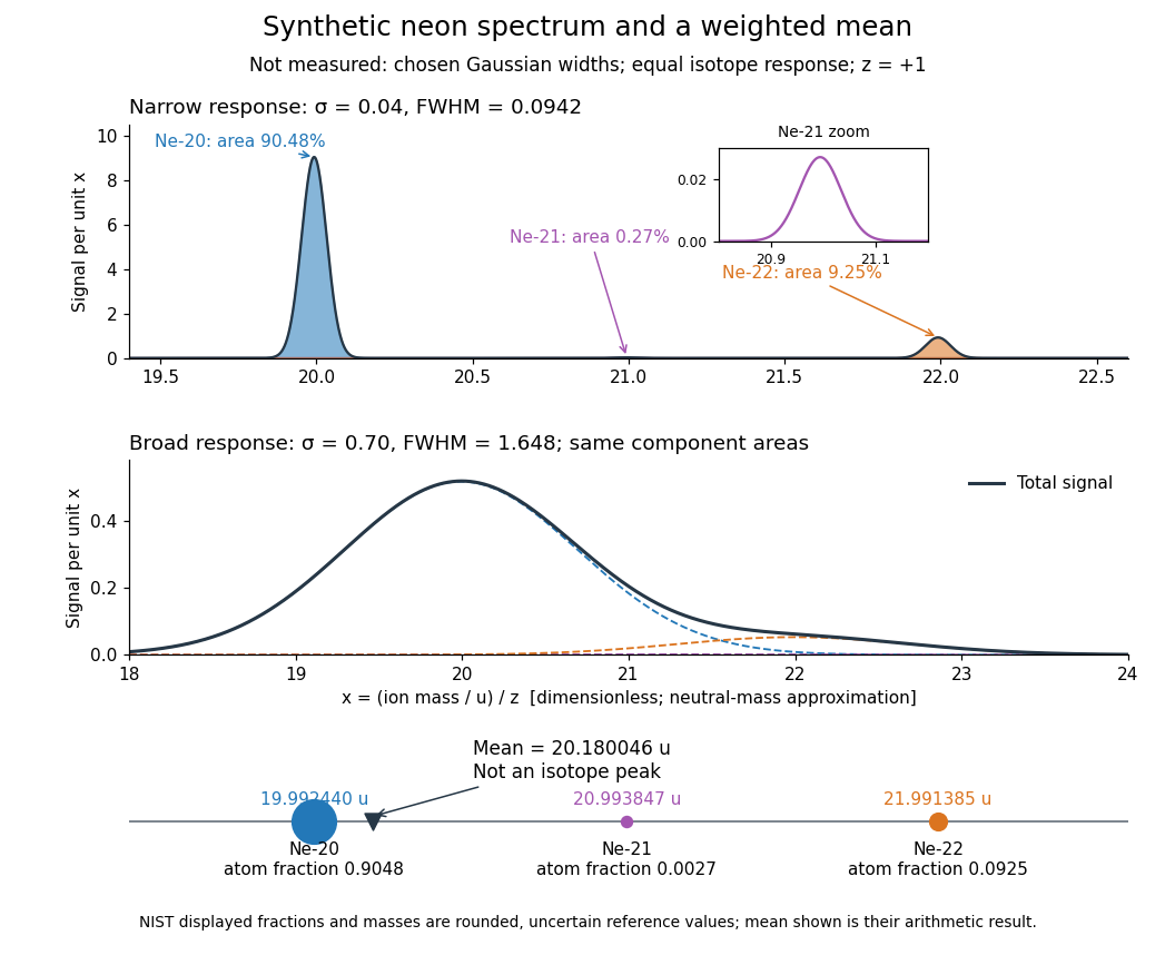
Broadening can hide a weak component without changing its area in this ideal model. An actual mass spectrum can also contain molecular ions, different electric charge states, background, and unequal detection responses. A missing visible peak therefore cannot by itself prove the absence of an isotope. Conversely, a fractional atomic weight is a property of a population: there is no requirement for an ion peak at the weighted mean.
The ratio of an ion's mass to its electric charge; in SI it has units . A convenient numerical mass spectrum coordinate is , with and positive integer here. This is dimensionless. Doubling at fixed mass halves , so the electric charge state must be identified before assigning an isotope.
A mass spectrometry instrument with a photographic readout. In the 1919 apparatus described in Chapter V: The Mass-Spectrograph, a gas discharge produced positive ions. Two narrow slits formed a ribbon beam in a vacuum; plates applied an electric field to spread it, an aperture selected part of it, and a magnetic field bent it oppositely. Focusing reduced the spread caused by differing ion speeds, concentrating a given mass-to-charge ratio into a line on a photographic plate.
The observed quantity was line displacement from a fiducial spot. Known reference lines calibrated displacement against mass-to-charge ratio; repeated exposures with changed magnetic field tested the calibration. Evacuation limited collisions. Comparing line shapes with narrow and wide apertures helped distinguish geometric broadening from photographic spreading. Finite slit widths, plate response, and overlapping molecular or multiply charged ions limited interpretation. See Chapter V: The Mass-Spectrograph (§§33–40: apparatus and photographic procedure; §§43 and 45–46: calibration, aperture comparisons, and accuracy).
In Mass spectra and isotopes by Francis William Aston (Nobel lecture, 12 December 1922), the reported neon lines at 20 and 22 have companions at 10 and 11 from doubly charged ions. That paired pattern and comparison with reference lines support different atomic masses within one chemical element, rather than an atomic mass concentrated at the bulk average. The lecture also describes an earlier failed separation by distillation and partial separation by diffusion, showing why the focused mass spectrum supplied stronger evidence. These numbers used a historical oxygen-based reference scale. The lecture's whole-number rule was an empirical approximation at its stated accuracy, not the modern exact definition .[ref]
Mass spectra and isotopes by Francis William Aston. pp. 9–13: separation attempts, focusing, reference lines, charge orders, and neon; pp. 15–17: whole-number rule and historical nuclear interpretation
Hydronium is the ion formed when a water molecule accepts a proton. It provides the usual aqueous shorthand for the hydrogen ion used in pH calculations.
In acid-base chemistry, hydrogen ion usually refers to positively charged hydrogen, represented by . In water, this notation describes solvated species, commonly represented by hydronium, rather than an isolated bare proton. The hydrogen ion thermodynamic activity defines pH.
Nearest-neighbor interpolation assigns each requested location the value of its nearest available sample, with a specified convention for ties. In lossy block averaging, samples are placed at block centres and each is copied into its four original pixel positions. This enlarges the raster image without recovering discarded detail.
Quantization maps numerical values to a specified discrete collection of representable values. In lossy block averaging, maps block arithmetic means in to eight-bit integers. Thus and . Different means can share a stored value, making this step irreversible.
A universal hash family is a finite collection of hash functions into an output set of size such that, for any fixed distinct inputs ,The choice of uses the uniform distribution on a finite set. The keys are fixed before that choice: the randomness belongs to the hash function, so the guarantee does not assume naturally random keys. Choose one member and keep it while using the table; changing it requires redistributing the stored records. The bound holds separately for every distinct pair, without requiring uniform individual outputs or independent random variables. A strongly universal hash family supplies those stronger properties.
The practical payoff follows from linearity of expectation. If stored keys are distinct from a fixed query, let count how many share its bucket. Then : each key contributes at most to the expected value. With stored keys and buckets, an unsuccessful search encounters at most one record on average over the random choice of hash function. This is an expected value, not a limit on every search; one unlucky choice can still create a long chain.
This calculation needs no independence between the collision events: linearity of expectation adds their individual probabilities. The fixed-query condition matters, since deliberately choosing keys after inspecting the selected hash function can target a crowded bucket.
Carter and Wegman introduced this way of analyzing storage and retrieval in their 1977 paper: average over a chosen class of hash functions while allowing any fixed sequence of inputs. Their 1979 journal version develops the same universal-pair collision condition and constructions. The insight is useful because a randomized algorithm can obtain a performance guarantee through its own choices, even when its inputs have inconvenient patterns.[ref]
https://dl.acm.org/doi/10.1145/800105.803400. Carter and Wegman, Universal classes of hash functions, STOC 1977
[ref]https://www.cs.princeton.edu/courses/archive/fall09/cos521/Handouts/universalclasses.pdf. Carter and Wegman, Universal Classes of Hash Functions, 1979
An almost strongly universal hash family relaxes the exact ordered pair balance of a strongly universal hash family. In the convention used here, choose with the uniform distribution on a finite set from a family with possible outputs. Every individual output remains uniform, and for every distinct pair of inputs and every specified ordered pair of outputs ,Equivalently, the conditional probability is at most . This asks how predictable a second output can become after the first is known.
For , strongly universal hash families give : learning one output leaves each specified second output with conditional probability . A looser guarantee permits a specified ordered pair to have probability as large as , while each individual output still has probability . Summing over the five equal ordered pairs bounds the collision probability by , rather than the required of a universal hash family. Thus an almost strongly universal hash family need not be a universal hash family. Necessarily , because the conditional probabilities sum to one; equality recovers a strongly universal hash family. This relaxation is useful in Wegman–Carter authentication, where efficiency can be traded against a quantified forgery bound within a complete message authentication protocol.
A hash collision is a function collision of a hash function : two distinct inputs have the same output, . Repeating the same input is not a hash collision. Unequal hash values prove the keys differ; equal hash values only identify candidates that might be equal. This makes a hash function useful as a compact filter before comparing the original data.
Here is a deliberately simple example using modular arithmetic. Let for nonnegative integer keys, and let a four-bucket hash table use the further bucket index . For keys , the hash values are , while all three bucket indices are . Thus and form a hash collision for ; and share a table bucket even though their full hash values differ. Always specify which function is being compared: a table collision concerns the bucket-index function, which may discard more information than the original hash function.
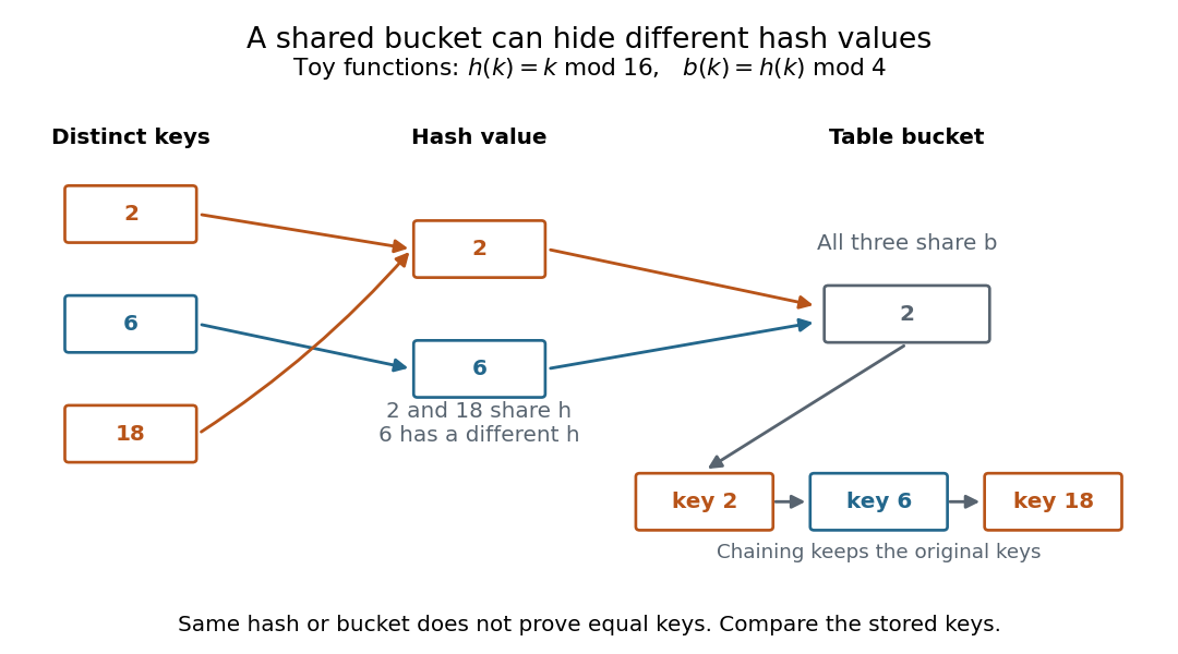
With separate chaining, bucket holds all three records in a linked list. A search for visits that bucket and compares the stored keys until it finds ; a search for visits the same bucket but rejects every stored key. A hash collision changes the search work, while key comparison preserves correctness. Storing only one record per hash value would incorrectly merge distinct keys. This is the purpose of collision handling in a hash table.[ref]
The pigeonhole principle explains inevitability: if a hash function has only possible outputs, any distinct inputs contain a hash collision. In particular, a function whose domain of a function is larger than its finite codomain cannot be an injective function. This is an existence statement; it gives neither an efficient way to find the pair nor a probability for a smaller collection of keys. A particular small collection might have no hash collision at all.
For a cryptographic hash function, collision resistance asks that finding any two distinct messages with equal full digests be computationally infeasible under the specified model and resources. It does not mean that hash collisions do not exist. Preimage resistance asks a different question: given a target digest , how hard is it to find a message with ? The collision finder may choose both messages and their common digest; the preimage finder is given the digest in advance. These definitions distinguish two search tasks, independently of how a hash table stores records.[ref]
https://nvlpubs.nist.gov/nistpubs/Legacy/SP/nistspecialpublication800-107r1.pdf. Quynh Dang, NIST SP 800-107 Revision 1 (2012), section 3.1 and section 4.1, definitions of collision and preimage resistance
In Newtonian gravity, the gravitational field specifies the acceleration of a freely falling test particle at each position. A gravitational potential gives , with the gradient taken in the spatial geometry of the model. In general relativity, the metric tensor describes gravitational effects, and tidal forces are encoded by spacetime curvature.
Population genetics studies the frequencies of alleles and genotypes in populations, and their changes through inheritance, mutation, selection, migration and random sampling. Kingman's coalescent describes a neutral sample's ancestry backward in time.
An allele is one of the alternative inherited states at a genetic locus, often distinguished by a difference in DNA sequence. A population can contain many alleles, although a two-copy diploid individual carries at most two at that genetic locus, one inherited from each parent. See NHGRI: allele.
Count copies, not just individuals, when computing allele frequency: in 100 individuals with genotype counts , , , there are copies of among 200, so . The heterozygotes contribute to both allele counts. This converts observed genotypes into the population quantity needed by the Hardy-Weinberg principle.
A genotype records the inherited alleles carried by an individual at one or more genetic loci. At a two-copy diploid genetic locus with alleles , the possible unordered genotypes are . The first and last are homozygotes; the middle is a heterozygote. The notation records inherited states, without yet asserting their phenotypes. See NHGRI: genotype.
An unordered combines the two parental orders and . This small bookkeeping point explains the factor two in Hardy-Weinberg proportions and in an cross. If parental origin or arrangement across several genetic loci matters, a phase-known genotype retains extra information about the two haplotypes.
A phenotype is an observable characteristic of an organism, arising from its genotype, environment and other influences. Seed shape is a phenotype; is a genotype. The distinction prevents appearance from being mistaken for a complete inherited description. See NHGRI: phenotype.
For a specified binary phenotype , let its penetrance in genotype be . The law of total probability gives . Thus the ideal example has : the familiar follows only when these penetrances are . A pedigree likelihood keeps inheritance and the conditional phenotype model as separate factors.
Pinned article: Introduction to the OurBigBook Project
Welcome to the OurBigBook Project! Our goal is to create the perfect publishing platform for STEM subjects, and get university-level students to write the best free STEM tutorials ever.
Everyone is welcome to create an account and play with the site: ourbigbook.com/go/register. We belive that students themselves can write amazing tutorials, but teachers are welcome too. You can write about anything you want, it doesn't have to be STEM or even educational. Silly test content is very welcome and you won't be penalized in any way. Just keep it legal!
Intro to OurBigBook
. Source. We have two killer features:
- topics: topics group articles by different users with the same title, e.g. here is the topic for the "Fundamental Theorem of Calculus" ourbigbook.com/go/topic/fundamental-theorem-of-calculusArticles of different users are sorted by upvote within each article page. This feature is a bit like:
- a Wikipedia where each user can have their own version of each article
- a Q&A website like Stack Overflow, where multiple people can give their views on a given topic, and the best ones are sorted by upvote. Except you don't need to wait for someone to ask first, and any topic goes, no matter how narrow or broad
This feature makes it possible for readers to find better explanations of any topic created by other writers. And it allows writers to create an explanation in a place that readers might actually find it.
Figure 1. Screenshot of the "Derivative" topic page. View it live at: ourbigbook.com/go/topic/derivativeVideo 2. OurBigBook Web topics demo. Source. - local editing: you can store all your personal knowledge base content locally in a plaintext markup format that can be edited locally and published either:This way you can be sure that even if OurBigBook.com were to go down one day (which we have no plans to do as it is quite cheap to host!), your content will still be perfectly readable as a static site.
- to OurBigBook.com to get awesome multi-user features like topics and likes
- as HTML files to a static website, which you can host yourself for free on many external providers like GitHub Pages, and remain in full control

Figure 2. You can publish local OurBigBook lightweight markup files to either OurBigBook.com or as a static website.
Figure 3. Visual Studio Code extension installation.
Figure 5. . You can also edit articles on the Web editor without installing anything locally. Video 3. Edit locally and publish demo. Source. This shows editing OurBigBook Markup and publishing it using the Visual Studio Code extension. 
- Infinitely deep tables of contents:




All our software is open source and hosted at: github.com/ourbigbook/ourbigbook
Further documentation can be found at: docs.ourbigbook.com
Feel free to reach our to us for any help or suggestions: docs.ourbigbook.com/#contact