
Incoming links: Discrete Fourier transform
The best articles by Ciro Santilli Updated 2025-07-16
These are the best articles ever authored by Ciro Santilli, most of them in the format of Stack Overflow answers.
Ciro posts update about new articles on his Twitter accounts.
Some random generally less technical in-tree essays will be present at: Section "Essays by Ciro Santilli".
- Trended on Hacker News:
- CIA 2010 covert communication websites on 2023-06-11. 190 points, a mild success.
- x86 Bare Metal Examples on 2019-03-19. 513 points. The third time something related to that repo trends. Hacker news people really like that repo!
- again 2020-06-27 (archive). 200 points, repository traffic jumped from 25 daily unique visitors to 4.6k unique visitors on the day
- How to run a program without an operating system? on 2018-11-26 (archive). 394 points. Covers x86 and ARM
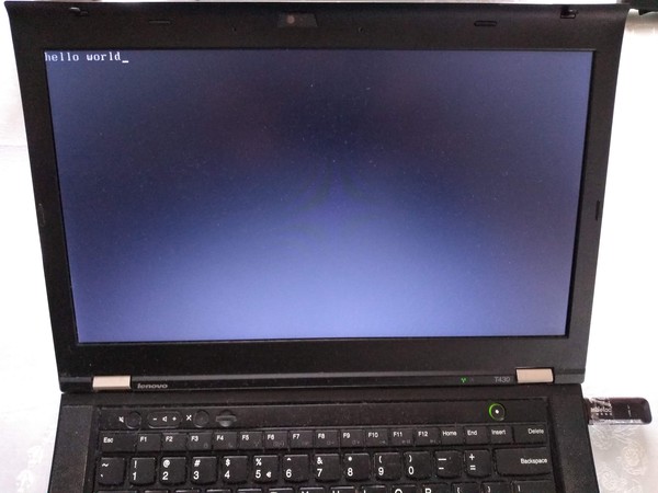
- ELF Hello World Tutorial on 2017-05-17 (archive). 334 points.
- x86 Paging Tutorial on 2017-03-02. Number 1 Google search result for "x86 Paging" in 2017-08. 142 points.
- x86 assembly
- What does "multicore" assembly language look like?
- What is the function of the push / pop instructions used on registers in x86 assembly? Going down to memory spills, register allocation and graph coloring.
- Linux kernel
- What do the flags in /proc/cpuinfo mean?
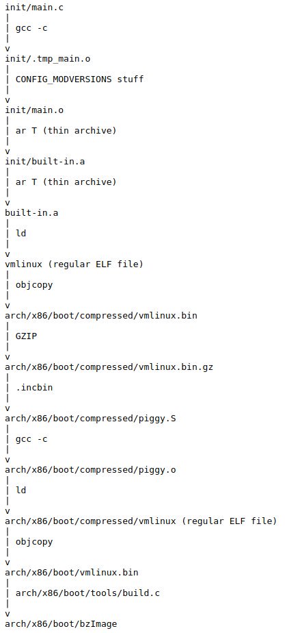
- How does kernel get an executable binary file running under linux?
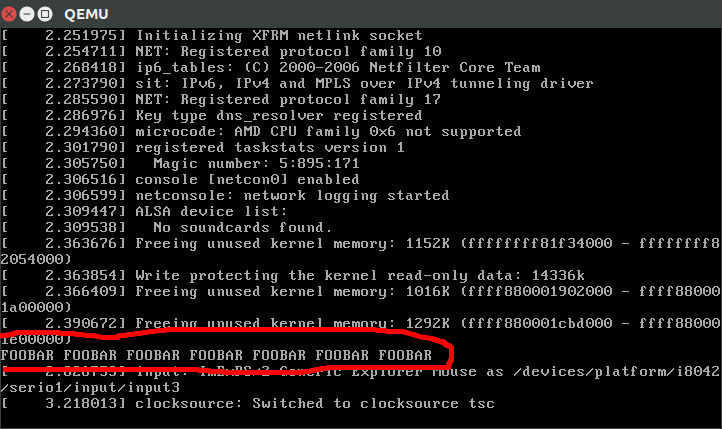
- How to debug the Linux kernel with GDB and QEMU?
- Can the sys_execve() system call in the Linux kernel receive both absolute or relative paths?
- What is the difference between the kernel space and the user space?
- Is there any API for determining the physical address from virtual address in Linux?
- Why do people write the
#!/usr/bin/envpython shebang on the first line of a Python script? - How to solve "Kernel Panic - not syncing: VFS: Unable to mount root fs on unknown-block(0,0)"?
- Single program Linux distro
- QEMU
- gcc and Binutils:
- How do linkers and address relocation works?
- What is incremental linking or partial linking?
- GOLD (
-fuse-ld=gold) linker vs the traditional GNU ld and LLVM ldd - What is the -fPIE option for position-independent executables in GCC and ld? Concrete examples by running program through GDB twice, and an assembly hello world with absolute vs PC relative load.
- How many GCC optimization levels are there?
- Why does GCC create a shared object instead of an executable binary according to file?
- C/C++: almost all of those fall into "disassemble all the things" category. Ciro also does "standards dissection" and "a new version of the standard is out" answers, but those are boring:
- What does "static" mean in a C program?
- In C++ source, what is the effect of
extern "C"? - Char array vs Char Pointer in C
- How to compile glibc from source and use it?
- When should
static_cast,dynamic_cast,const_castandreinterpret_castbe used? - What exactly is
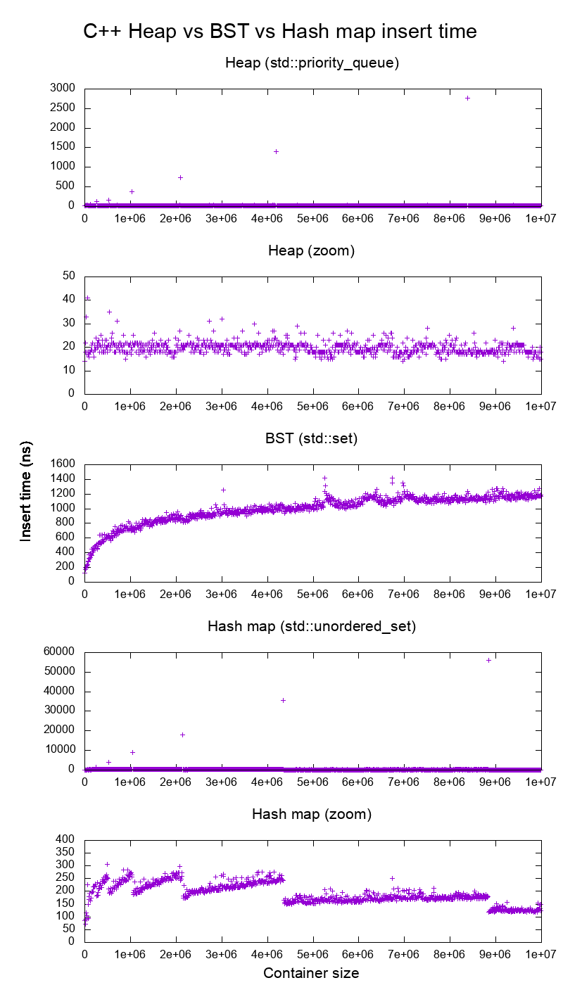
std::atomicin C++?. This answer was originally more appropriately entitled "Let's disassemble some stuff", and got three downvotes, so Ciro changed it to a more professional title, and it started getting upvotes. People judge books by their covers. notmain.o 0000000000000000 0000000000000017 W MyTemplate<int>::f(int) main.o 0000000000000000 0000000000000017 W MyTemplate<int>::f(int)Code 1.. From: What is explicit template instantiation in C++ and when to use it?nmoutputs showing that objects are redefined multiple times across files if you don't use template instantiation properly
- IEEE 754
- What is difference between quiet NaN and signaling NaN?
- In Java, what does NaN mean?
Without subnormals:

          +---+---+-------+---------------+-------------------------------+
exponent  | ? | 0 |   1   |       2       |               3               |
          +---+---+-------+---------------+-------------------------------+
          |   |   |       |               |                               |
          v   v   v       v               v                               v
          -----------------------------------------------------------------
floats    *    **** * * * *   *   *   *   *       *       *       *       *
          -----------------------------------------------------------------
          ^   ^   ^       ^               ^                               ^
          |   |   |       |               |                               |
          0   |   2^-126  2^-125          2^-124                          2^-123
              |
              2^-127

With subnormals:

          +-------+-------+---------------+-------------------------------+
exponent  |   0   |   1   |       2       |               3               |
          +-------+-------+---------------+-------------------------------+
          |       |       |               |                               |
          v       v       v               v                               v
          -----------------------------------------------------------------
floats    * * * * * * * * *   *   *   *   *       *       *       *       *
          -----------------------------------------------------------------
          ^   ^   ^       ^               ^                               ^
          |   |   |       |               |                               |
          0   |   2^-126  2^-125          2^-124                          2^-123
              |
              2^-127
- Computer science
- Algorithms
- Is it necessary for NP problems to be decision problems?
- Polynomial time and exponential time. Answered focusing on the definition of "exponential time".
- What is the smallest Turing machine where it is unknown if it halts or not?. Answer focusing on "blank tape" initial condition only. Large parts of it are summarizing the Busy Beaver Challenge, but some additions were made.
- Algorithms
- Git
| 0 | 4 | 8 | C | |-------------|--------------|-------------|----------------| 0 | DIRC | Version | File count | ctime ...| 0 | ... | mtime | device | 2 | inode | mode | UID | GID | 2 | File size | Entry SHA-1 ...| 4 | ... | Flags | Index SHA-1 ...| 4 | ... |tree {tree_sha} {parents} author {author_name} <{author_email}> {author_date_seconds} {author_date_timezone} committer {committer_name} <{committer_email}> {committer_date_seconds} {committer_date_timezone} {commit message}- How do I clone a subdirectory only of a Git repository?
- Python
- Web technology
- OpenGL
- Node.js
- Ruby on Rails
- POSIX
- What is POSIX? Huge classified overview of the most important things that POSIX specifies.
- Systems programming
- What do the terms "CPU bound" and "I/O bound" mean?
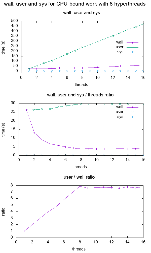
Figure 12. Plot of "real", "user" and "sys" mean times of the output of time for CPU-bound workload with 8 threads. Source. From: What do 'real', 'user' and 'sys' mean in the output of time?+--------+ +------------+ +------+ | device |>---------------->| function 0 |>----->| BAR0 | | | | | +------+ | |>------------+ | | | | | | | +------+ ... ... | | |>----->| BAR1 | | | | | | +------+ | |>--------+ | | | +--------+ | | ... ... ... | | | | | | | | +------+ | | | |>----->| BAR5 | | | +------------+ +------+ | | | | | | +------------+ +------+ | +--->| function 1 |>----->| BAR0 | | | | +------+ | | | | | | +------+ | | |>----->| BAR1 | | | | +------+ | | | | ... ... ... | | | | | | +------+ | | |>----->| BAR5 | | +------------+ +------+ | | | ... | | | +------------+ +------+ +------->| function 7 |>----->| BAR0 | | | +------+ | | | | +------+ | |>----->| BAR1 | | | +------+ | | ... ... ... | | | | +------+ | |>----->| BAR5 | +------------+ +------+Code 5.Logical struture PCIe device, functions and BARs. From: What is the Base Address Register (BAR) in PCIe?
- Electronics
- Raspberry Pi

Figure 13. . Image from answer to: How to hook up a Raspberry Pi via Ethernet to a laptop without a router? 
Figure 14. . Image from answer to: How to hook up a Raspberry Pi via Ethernet to a laptop without a router? 
Figure 15. . Image from answer to: How to emulate the Raspberry Pi 2 on QEMU? 
Figure 16. . Image from answer to: How to run a C program with no OS on the Raspberry Pi?
- Raspberry Pi
- Computer security
- Media
Video 2. . Source. The original question was deleted, lol...: How to programmatically synthesize music?- How to resize a picture using ffmpeg's sws_scale()?
- Is there any decent speech recognition software for Linux? ran a few examples manually on
vosk-apiand compared to ground truth.
- Eclipse
- Computer hardware
- Scientific visualization software
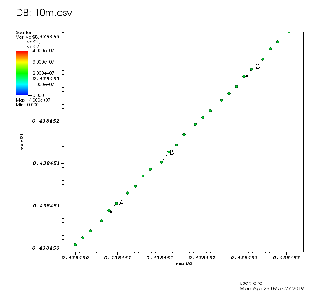
Figure 17. VisIt zoom in 10 million straight line plot with some manually marked points. Source. From: Section "Survey of open source interactive plotting software with a 10 million point scatter plot benchmark by Ciro Santilli"
- Numerical analysis
Video 3. Real-time heat equation OpenGL visualization with interactive mouse cursor using relaxation method by Ciro Santilli (2016)Source.
- Computational physics
- Register transfer level languages like Verilog and VHDL
- Verilog:
Figure 19. . See also: Section "Verilator interactive example"
- Verilog:
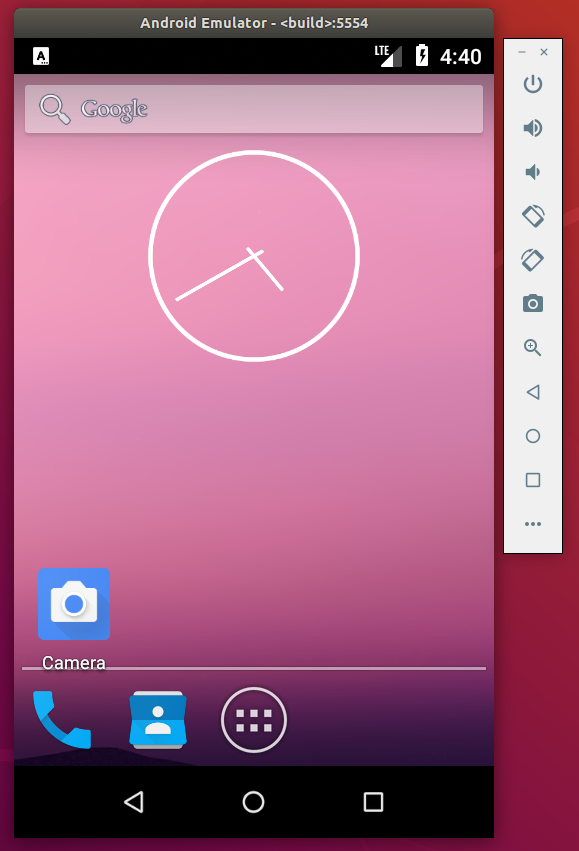
- Android
- Debugging
- Program optimization
- What is tail call optimization?

Figure 21. . Source. The answer compares gprof, valgrind callgrind, perf and gperftools on a single simple executable.
- Data
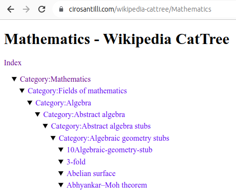
Figure 22. Mathematics dump of Wikipedia CatTree. Source. In this project, Ciro Santilli explored extracting the category and article tree out of the Wikipedia dumps.
- Mathematics

Figure 23. Diagram of the fundamental theorem on homomorphisms by Ciro Santilli (2020)Shows the relationship between group homomorphisms and normal subgroups.- Section "Formalization of mathematics": some early thoughts that could be expanded. Ciro almost had a stroke when he understood this stuff in his teens.

Figure 24. Simple example of the Discrete Fourier transform. Source. That was missing from Wikipedia page: en.wikipedia.org/wiki/Discrete_Fourier_transform!
- Network programming
- Physics
- Biology
- Quantum computing
- Section "Quantum computing is just matrix multiplication"

Figure 28. Visualization of the continuous deformation of states as we walk around the Bloch sphere represented as photon polarization arrows. From: Understanding the Bloch sphere.
- Bitcoin
- GIMP

Figure 29. GIMP screenshot part of how to combine two images side-by-side in GIMP?.
- Home DIY

Figure 30. Total_Blackout_Cassette_Roller_Blind_With_Curtains.Source. From: Section "How to blackout your window without drilling"
- China


Deletionism on Wikipedia Updated 2025-07-16
Some examples by Ciro Santilli follow.
Of the tutorial-subjectivity type:
- This edit perfectly summarizes how Ciro feels about Wikipedia (no particular hate towards that user, he was a teacher at the prestigious Pierre and Marie Curie University and actually as a wiki page about him):which removed the only diagram that was actually understandable to non-Mathematicians, which Ciro Santilli had created, and received many upvotes at: math.stackexchange.com/questions/776039/intuition-behind-normal-subgroups/3732426#3732426. The removal does not generate any notifications to you unless you follow the page which would lead to infinite noise, and is extremely difficult to find out how to contact the other person. The removal justification is even somewhat ad hominem: how does he know Ciro Santilli is also not a professional Mathematician? :-) Maybe it is obvious because Ciro explains in a way that is understandable. Also removal makes no effort to contact original author. Of course, this is caused by the fact that there must also have been a bunch of useless edits not done by Ciro, and there is no reputation system to see if you should ignore a person or not immediately, so removal author has no patience anymore. This is what makes it impossible to contribute to Wikipedia: your stuff gets deleted at any time, and you don't know how to appeal it. Ciro is going to regret having written this rant after Daniel replies and shows the diagram is crap. But that would be better than not getting a reply and not learning that the diagram is crap.
rm a cryptic diagram (not understandable by a professional mathematician, without further explanations
- en.wikipedia.org/w/index.php?title=Finite_field&type=revision&diff=1044934168&oldid=1044905041 on finite fields with edit comment "Obviously: X ≡ α". Discussion at en.wikipedia.org/wiki/Talk:Finite_field#Concrete_simple_worked_out_example Some people simply don't know how to explain things to beginners, or don't think Wikipedia is where it should be done. One simply can't waste time fighting off those people, writing good tutorials is hard enough in itself without that fight.
- en.wikipedia.org/w/index.php?title=Discrete_Fourier_transform&diff=1193622235&oldid=1193529573 by user Bob K. removed Ciro Santilli's awesome simple image of the Discrete Fourier transform as seen at en.wikipedia.org/w/index.php?title=Discrete_Fourier_transform&oldid=1176616763:with message:
Hello. I am a retired electrical engineer, living near Washington,DC. Most of my contributions are in the area of DSP, where I have about 40 years of experience in applications on many different processors and architectures.
Thank you so much!!remove non-helpful image
Maybe it is a common thread that these old "experts" keep removing anything that is actually intelligible by beginners? Section "There is value in tutorials written by beginners"Also ranted at: x.com/cirosantilli/status/1808862417566290252
Figure 1. Source at: numpy/fft_plot.py. - when Ciro Santilli created Scott Hassan's page, he originally included mentions of his saucy divorce: en.wikipedia.org/w/index.php?title=Scott_Hassan&oldid=1091706391 These were reverted by Scott's puppets three times, and Ciro and two other editors fought back. Finally, Ciro understood that Hassan's puppets were likely right about the removal because you can't talk about private matters of someone who is low profile:even if it is published in well known and reliable publications like the bloody New York Times. In this case, it is clear that most people wanted to see this information summarized on Wikipedia since others fought back Hassan's puppet. This is therefore a failure of Wikipedia to show what the people actually want to read about.This case is similar to the PsiQuantum one. Something is extremely well known in an important niche, and many people want to read about it. But because the average person does not know about this important subject, and you are limited about what you can write about it or not, thus hurting the people who want to know about it.
Notability constraints, which are are way too strict:There are even a Wikis that were created to remove notability constraints: Wiki without notability requirements.
- even information about important companies can be disputed. E.g. once Ciro Santilli tried to create a page for PsiQuantum, a startup with $650m in funding, and there was a deletion proposal because it did not contain verifiable sources not linked directly to information provided by the company itself: en.wikipedia.org/wiki/Wikipedia:Articles_for_deletion/PsiQuantum Although this argument is correct, it is also true about 90% of everything that is on Wikipedia about any company. Where else can you get any information about a B2B company? Their clients are not going to say anything. Lawsuits and scandals are kind of the only possible source... In that case, the page was deleted with 2 votes against vs 3 votes for deletion.is very similar to Stack Exchange's own Stack Overflow content deletion issues. Ain't Nobody Got Time For That. "Ain't Nobody Got Time for That" actually has a Wiki page: en.wikipedia.org/wiki/Ain%27t_Nobody_Got_Time_for_That. That's notable. Unlike a $600M+ company of course.
should we delete this extremely likely useful/correct content or not according to this extremely complex system of guidelines"
In December 2023 the page was re-created, and seemed to stick: en.wikipedia.org/wiki/Talk:PsiQuantum#Secondary_sources It's just a random going back and forth. Author Ctjk has an interesting background:I am a legal official at a major government antitrust agency. The only plausible connection is we regulate tech firms
For these reasons reason why Ciro basically only contributes images to Wikipedia: because they are either all in or all out, and you can determine which one of them it is. And this allows images to be more attributable, so people can actually see that it was Ciro that created a given amazing image, thus overcoming Wikipedia's lack of reputation system a little bit as well.
Wikipedia is perfect for things like biographies, geography, or history, which have a much more defined and subjective expository order. But when it comes to "tutorials of how to actually do stuff", which is what mathematics and physics are basically about, Wikipedia has a very hard time to go beyond dry definitions which are only useful for people who already half know the stuff. But to learn from zero, newbies need tutorials with intuition and examples.
Bibliography:
- gwern.net/inclusionism from gwern.net:
Iron Law of Bureaucracy: the downwards deletionism spiral discourages contribution and is how Wikipedia will die.
- Quote "Golden wiki vs Deletionism on Wikipedia"
Discrete Fourier transform Updated 2025-07-16
Output: another sequence of complex numbers such that:Intuitively, this means that we are braking up the complex signal into sinusoidal frequencies:and is the amplitude of each sine.
- : is kind of magic and ends up being a constant added to the signal because
- : sinusoidal that completes one cycle over the signal. The larger the , the larger the resolution of that sinusoidal. But it completes one cycle regardless.
- : sinusoidal that completes two cycles over the signal
- ...
- : sinusoidal that completes cycles over the signal
Motivation: similar to the Fourier transform:In particular, the discrete Fourier transform is used in signal processing after a analog-to-digital converter. Digital signal processing historically likely grew more and more over analog processing as digital processors got faster and faster as it gives more flexibility in algorithm design.
- compression: a sine would use N points in the time domain, but in the frequency domain just one, so we can throw the rest away. A sum of two sines, only two. So if your signal has periodicity, in general you can compress it with the transform
- noise removal: many systems add noise only at certain frequencies, which are hopefully different from the main frequencies of the actual signal. By doing the transform, we can remove those frequencies to attain a better signal-to-noise
Sample software implementations:
- numpy.fft, notably see the example: numpy/fft.py
DFT of with 25 points
. This is a simple example of a discrete Fourier transform for a real input signal. It illustrates how the DFT takes N complex numbers as input, and produces N complex numbers as output. It also illustrates how the discrete Fourier transform of a real signal is symmetric around the center point. Fast Fourier transform Updated 2025-07-16
An efficient algorithm to calculate the discrete Fourier transform.
numpy/fft.py Updated 2025-07-16
Output:With our understanding of the discrete Fourier transform we see clearly that:
sin(t)
fft
real 0 0 0 0 0 0 0 0 0 0 0 0 0 0 0 0 0 0 0 0
imag 0 -10 0 0 0 0 0 0 0 0 0 0 0 0 0 0 0 0 0 10
rfft
real 0 0 0 0 0 0 0 0 0 0 0
imag 0 -10 0 0 0 0 0 0 0 0 0

sin(t) + sin(4t)
fft
real 0 0 0 0 0 0 0 0 0 0 0 0 0 0 0 0 0 0 0 0
imag 0 -10 0 0 -10 0 0 0 0 0 0 0 0 0 0 0 10 0 0 10
rfft
real 0 0 0 0 0 0 0 0 0 0 0
imag 0 -10 0 0 -10 0 0 0 0 0 0- the signal is being decomposed into sinusoidal components
- because we are doing the Discrete Fourier transform of a real signal, for the
fft, so there is redundancy in the. We also understand thatrfftsimply cuts off and only keeps half of the coefficients
qiskit/qft.py Updated 2025-07-16
This is an example of the
qiskit.circuit.library.QFT implementation of the Quantum Fourier transform function which is documented at: docs.quantum.ibm.com/api/qiskit/0.44/qiskit.circuit.library.QFTOutput:So this also serves as a more interesting example of quantum compilation, mapping the
init: [1, 0, 0, 0, 0, 0, 0, 0]
qc
     ┌──────────────────────────────┐┌──────┐
q_0: ┤0                             ├┤0     ├
     │                              ││      │
q_1: ┤1 Initialize(1,0,0,0,0,0,0,0) ├┤1 QFT ├
     │                              ││      │
q_2: ┤2                             ├┤2     ├
     └──────────────────────────────┘└──────┘
transpiled qc
     ┌──────────────────────────────┐                                     ┌───┐
q_0: ┤0                             ├────────────────────■────────■───────┤ H ├─X─
     │                              │              ┌───┐ │        │P(π/2) └───┘ │
q_1: ┤1 Initialize(1,0,0,0,0,0,0,0) ├──────■───────┤ H ├─┼────────■─────────────┼─
     │                              │┌───┐ │P(π/2) └───┘ │P(π/4)                │
q_2: ┤2                             ├┤ H ├─■─────────────■──────────────────────X─
     └──────────────────────────────┘└───┘
Statevector([0.35355339+0.j, 0.35355339+0.j, 0.35355339+0.j,
             0.35355339+0.j, 0.35355339+0.j, 0.35355339+0.j,
             0.35355339+0.j, 0.35355339+0.j],
            dims=(2, 2, 2))

init: [0.0, 0.35355339059327373, 0.5, 0.3535533905932738, 6.123233995736766e-17, -0.35355339059327373, -0.5, -0.35355339059327384]
Statevector([ 7.71600526e-17+5.22650714e-17j,
              1.86749130e-16+7.07106781e-01j,
             -6.10667421e-18+6.10667421e-18j,
              1.13711443e-16-1.11022302e-16j,
              2.16489014e-17-8.96726857e-18j,
             -5.68557215e-17-1.11022302e-16j,
             -6.10667421e-18-4.94044770e-17j,
             -3.30200457e-16-7.07106781e-01j],
dims=(2, 2, 2))QFT gate to Qiskit Aer primitives.If we don't
transpile in this example, then running blows up with:qiskit_aer.aererror.AerError: 'unknown instruction: QFT'The second input is:and the output of that approximately:which can be defined simply as the normalized DFT of the input quantum state vector.
[0, 1j/sqrt(2), 0, 0, 0, 0, 0, 1j/sqrt(2)]From this we see that the Quantum Fourier transform is equivalent to a direct discrete Fourier transform on the quantum state vector, related: physics.stackexchange.com/questions/110073/how-to-derive-quantum-fourier-transform-from-discrete-fourier-transform-dft