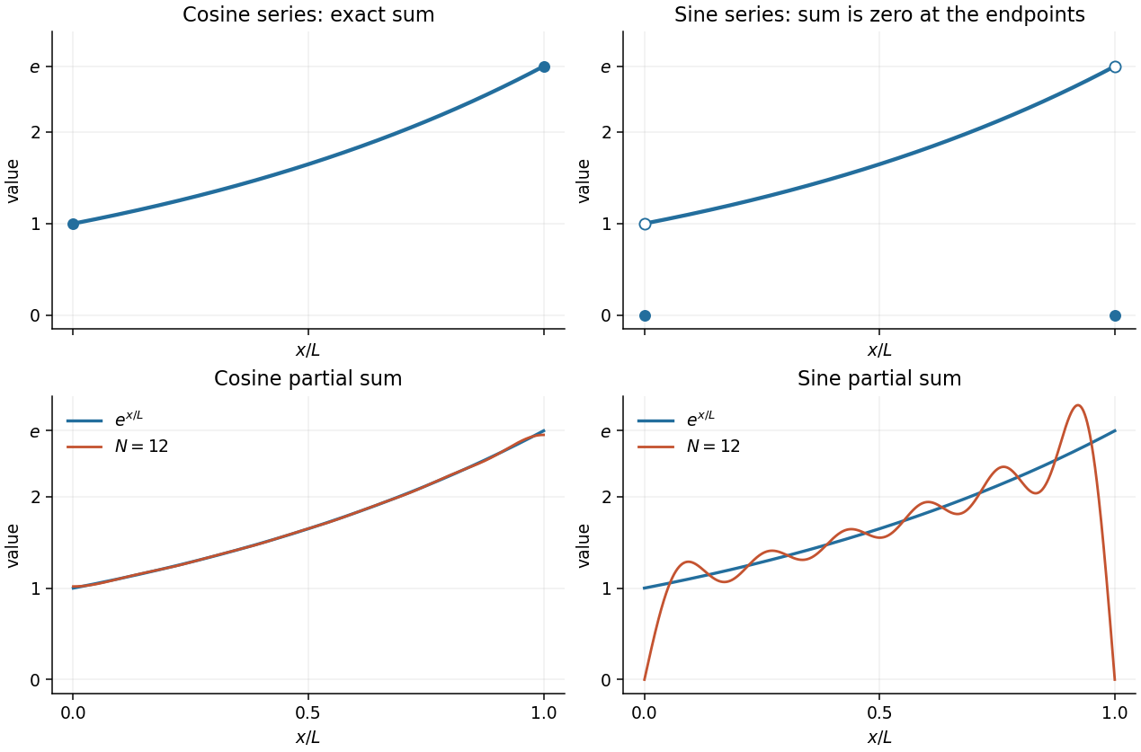
First, the Fourier coefficients of the Fourier cosine series decay as $O(n^{-2})$, whereas those of the Fourier sine series are of order $n^{-1}$. In particular, the absolute convergence bound for the Fourier cosine series gives a uniform tail estimateThus its tail is absolutely controlled using fewer Fourier harmonics. The Fourier sine series does not have an absolutely summable sequence of Fourier coefficients.

Second, the even extension is continuous, so its Fourier cosine series converges uniformly on the closed interval and approximates the nonzero endpoint limits correctly. The odd periodic extension has jumps, producing the Gibbs phenomenon in its Fourier sine series near zero and $L$. Every Fourier sine series partial sum is zero at both endpoints, so by approaching $L$ from inside $(0,L)$ one obtainsHence the Fourier sine series approximation cannot converge uniformly even on the whole open interval, despite pointwise convergence at each interior point. The Fourier cosine series approximation has faster coefficient decay and avoids the persistent errors near the endpoints.

Set $u=x/L$ and $q=n\pi$. The required integrals follow fromConsequently the Fourier coefficients areThus the Fourier cosine series isand its sum is $e^{x/L}$ everywhere on $[0,L]$. The Fourier sine series isand its sum is $e^{x/L}$ on $(0,L)$ and zero at the two endpoints. The open and filled circles in the sketches distinguish these endpoint limits from the actual values of the sum.

Under the stated piecewise smooth hypotheses, the Dirichlet convergence theorem for Fourier series gives the average of the two one-sided limits of the corresponding periodic extension. The even extension is continuous at both endpoints, so the Fourier cosine series converges toThe odd extension agrees with $f$ on $(0,L)$, but its left and right limits are $-f(0),f(0)$ at zero and $f(L),-f(L)$ at the join $L$. Therefore the Fourier sine series converges toIndeed every partial sum of the Fourier sine series is already zero at both endpoints. The endpoint values agree with $f$ only when the corresponding boundary values vanish.

The Fourier cosine series on $[0,L]$ isIt is the Fourier series of the even extension to $[-L,L]$, repeated with period $2L$. The Fourier sine series isIt comes from the odd extension and its $2L$-periodic extension. These Fourier coefficient formulas follow by Fourier orthogonality, since every nonconstant sine or cosine has squared integral $L/2$ on $[0,L]$, while the constant function has squared integral $L$.

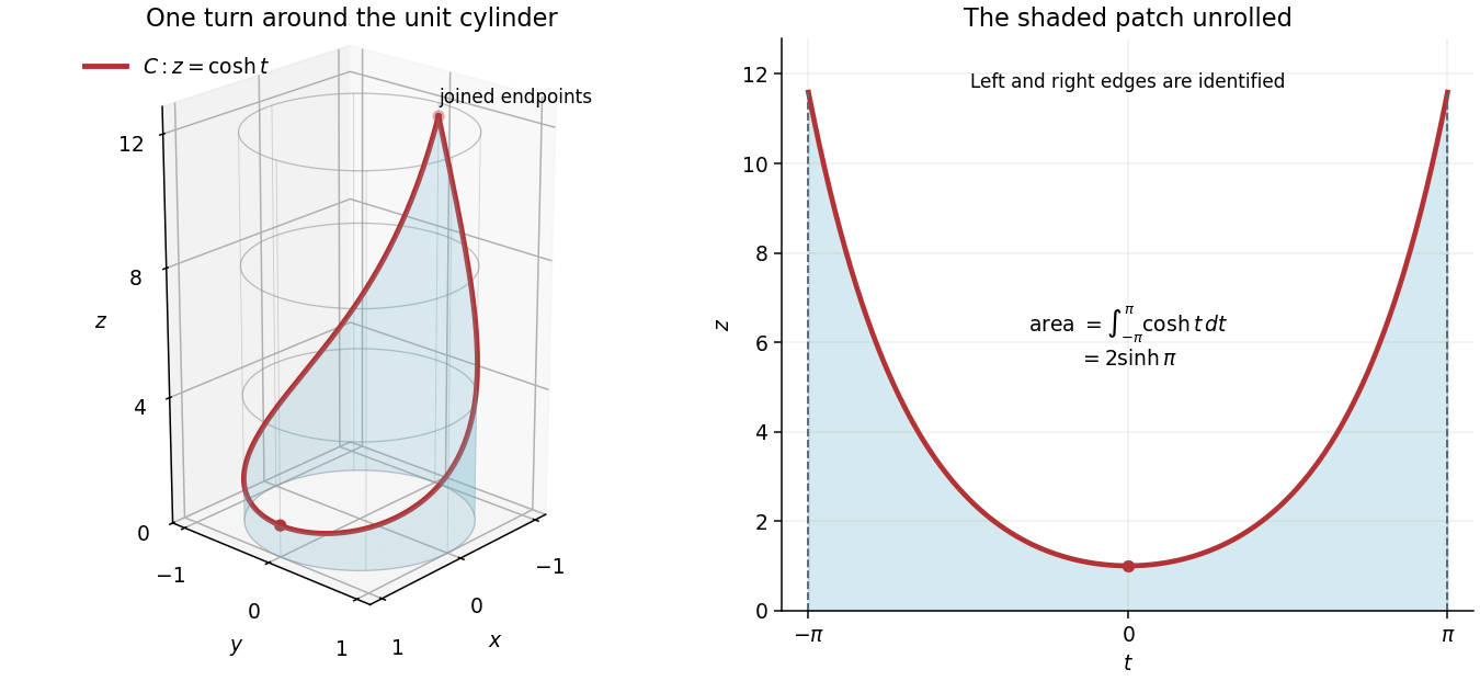
Parametrize the finite cylindrical surface patch byThe surface area element is $|{\mathbf{R}}_t\times {\mathbf{R}}_z|dtdz=dtdz$. The seam $t=\pm \pi$ has zero surface area, so it causes no overcounting. ThereforeUnrolling the unit circular cylinder preserves surface area, which explains the equality with the area under the hyperbolic cosine in the figure. The patch consists of the cylindrical surface alone; no flat base is included.

The velocity vector of the parametric curve isIts speed iswhere $\cosh t>0$ fixes the sign of the square root. Hence the arc length isThe coincidence of the endpoints does not duplicate any positive arc length.

For the given wrapped hyperbolic cosine curve,so $\boxed{C\subset S}$. The curve makes one full turn around the circular cylinder, descending from $(-1,0,\cosh \pi )$ to $(1,0,1)$ and ascending to its initial point. Its two parameter endpoints coincide; their tangent vectors $(0,-1,-\sinh \pi )$ and $(0,-1,\sinh \pi )$ do not agree, so the resulting closed curve has a corner there.

True. Two applications of Green's identities, or two integrations by parts, giveThe biharmonic equation makes the left side zero, while the two clamped boundary conditions $u={\partial }_{n}u=0$ annihilate the boundary integral. Consequentlyso $\Delta u=0$. Apply the first of Green's identities once more with $\varphi =\psi =u$: because $u=0$ on the boundary, it gives ${\int }_V|\nabla u{|}^2=0$. By path connectedness, $u$ is constant, and the zero boundary value implies $\boxed{u=0}$. This argument assumes the classical differentiability needed for the displayed integrations by parts.

False. Take $V=\{x^2+y^2+z^2<1\}$, the open unit ball, and $u(x,y,z)=x$. This is a nonzero harmonic function. On the unit sphere, the outward unit normal vector is $\mathbf{n}=(x,y,z)$, soThus the prescribed Robin boundary condition holds. Unlike the preceding case, Green's identities now give ${\int }_V|\nabla u{|}^2={\int }_{\partial V}{u}^2$, which permits nonzero solutions of the differential equation.

True. The first of Green's identities and the Robin boundary condition ${\partial }_{n}u=-u$ giveBoth integrands are nonnegative, so $\nabla u=0$ in $V$ and $u=0$ on the boundary. By path connectedness, $u$ is a constant function, and its boundary value makes that constant zero. Therefore $\boxed{u=0}$.

False. The constant function $u=1$ is a harmonic function and has zero normal derivative on every smooth boundary, but it is nonzero in $V$.

In fact, the first of Green's identities givesHence $\nabla u=0$; path connectedness makes $u$ constant throughout $V$. Thus this homogeneous Neumann boundary condition determines a harmonic function only up to an additive constant.

Choose $\mathbf{F}=\nabla \psi$ in the preceding product rule and apply the divergence theorem. Since $\nabla \cdot \nabla \psi =\Delta \psi$, this gives the first of Green's identities:Here ${\partial }_n\psi =\mathbf{n}\cdot \nabla \psi$ is the outward normal derivative. Interchange $\varphi$ and $\psi$, then subtract. The gradient dot products cancel, yielding the second of Green's identities:For example, $\varphi ,\psi \in C^2(\overline{V})$ with the needed extensions suffice for these applications of the divergence theorem.

Apply the product rule to each vector component and sum:Thus the divergence of a scalar field times a vector field contains a divergence term and a dot product with the gradient of the scalar field.

For a continuously differentiable vector field $\mathbf{F}$ on a neighborhood of the closure of $V$, the divergence theorem statesHere $\mathbf{n}$ is the outward unit normal vector; the right side is the outward flux through the boundary.

Use source spherical coordinates with radius $s$, polar angle $\alpha$ measured from the positive $z$-axis, and azimuth $\theta$. The lower half of the spherical shell has $a\le s\le 2a$, $\pi /2\le \alpha \le \pi$, and $0\le \theta \le 2\pi$. Its volume element is $s^2\sin \alpha dsd\alpha d\theta$. At the observation point $(0,0,h)$, $h>0$, the separation is $\sqrt{s^2+h^2-2sh\cos \alpha }$, soThe angular integral is elementary: put $q=\cos \alpha$ to obtainWe used $\sqrt{(s+h{)}^2}=s+h$ since both $s,h$ are positive. HenceThus the axial potential of a uniform hemispherical shell, at every point of the positive $z$-axis, isThere is no need to split into $h<a$, $a<h<2a$, and $h>2a$: the observation point is outside the lower hemisphere in all three cases. As checks, $\varphi (h)\to -3\pi G\rho a^2$ as $h\downarrow 0$, and at large $h$,The last factor is exactly the total mass of the lower half of the spherical shell.

Use source polar coordinates $x^{\prime }=s\cos \theta$, $y^{\prime }=s\sin \theta$ on the semicircular disk, with $0\le s\le a$ and $0\le \theta \le \pi$. Its surface area element is $sdsd\theta$, and the separation from $(0,0,h)$ is $\sqrt{s^2+h^2}$. ThusThis Newtonian gravitational potential is half that of the full disk because the separation is independent of the polar angle. At large $h$ it approaches $-G(\pi a^2\sigma /2)/h$, with the correct total mass.

Write the observation point as $(0,0,h)$ with $h>0$, reserving source coordinates for the integral. For the straight segment, $d{s}^{\prime }=d{x}^{\prime }$ and the separation is $\sqrt{x^{\prime 2}+h^2}$. Therefore its Newtonian gravitational potential isEquivalently $\varphi (h)=-2G\gamma \mathrm{arsinh}(a/h)$. At large $h$ it approaches $-G(2a\gamma )/h$, the Newtonian potential of a point mass with the segment's total mass.

For a volume source of constant mass density $\rho$, use $dm=\rho d{V}^{\prime }$. Its Newtonian gravitational potential is the volume integralThe source and observation position vectors are ${\mathbf{r}}^{\prime }$ and $\mathbf{r}$, respectively; $G$ is the gravitational constant. With this sign convention positive source mass gives negative Newtonian gravitational potential.

For the surface, a source element has mass $dm=\sigma d{S}^{\prime }$. Superposing its Newtonian gravitational potential gives the surface integralHere $d{S}^{\prime }$ is the source surface area element, ${\mathbf{r}}^{\prime }$ the source position vector, and $G$ the gravitational constant. The same zero-at-infinity convention applies.

Use the convention that the Newtonian gravitational potential tends to zero at infinity and the gravitational field is $-\nabla \varphi$. A source element of mass $dm$ at position vector ${\mathbf{r}}^{\prime }$ contributes $-Gdm/|\mathbf{r}-{\mathbf{r}}^{\prime }|$, where $G$ is the gravitational constant. For the curve, $dm=\gamma d{s}^{\prime }$, soHere $d{s}^{\prime }$ is arc length along the source curve; the expression is finite away from it. This normalization fixes the otherwise arbitrary additive constant.