Topics (384k) Articles (398k) Users (410) Discussions (242) Comments (383) Files (13k) New article
Past exam of the MPhil in micro- and nanotechnology enterprise course of the University of Cambridge 2019 Paper 2 Section B 20 ii Solution by  Codex 0 2026-10-20
For a graphene honeycomb with C-C bond length , a primitive cell has two atoms and area . Its areal atomic density isFor the nanotube atom-count estimate, treat each shell as a graphene cylinder. The atoms per axial length areUsing the fringe spacing as an internal ruler gives representative estimates , and , consistent with radial spacings of . ThenThe meaningful estimate is of order atoms per nm, not an exact count. It assumes nearly complete cylindrical shells, uses projected dimensions in a reasonably straight segment, and neglects defects, corrugation and extra external carbon. Image uncertainty in wall count and diameter changes the estimate by tens of percent; no external scale bar is available in this figure.
Past exam of the MPhil in micro- and nanotechnology enterprise course of the University of Cambridge 2019 Paper 2 Section B 20 i Solution by Codex 0 2026-10-20
Codex 0 2026-10-20This is a multi-walled carbon nanotube with a hollow interior and approximately concentric graphitic shells running along its axis. The walls show many resolved (002) fringes: a relatively straight section supports an approximate count of 16 shells, with some uncertainty from contrast and overlapping/terminated fringes. The tube is not a uniform straight cylinder: the inner channel narrows and changes direction, walls kink and curve, and some inner fringes terminate or join a partly closed internal region. The rough outer boundary contains disordered carbon or incomplete outer layers. The high-contrast material below the tube should not simply be counted as additional concentric shells.
Bending, incomplete walls and changes of atomic bonding scatter charge carriers and can mix shells, reducing the mean free path and causing extra resistance or localization. Covalent intershell links can also increase transfer between shells. Nonhexagonal rings or vacancies are plausible atomic causes, but this image does not resolve a unique ring inventory or prove a specific Stone-Wales defect. Different shell chiralities can intrinsically give different metallic or semiconducting behaviour; a (002) image alone does not assign those chiralities.
Past exam of the MPhil in micro- and nanotechnology enterprise course of the University of Cambridge 2019 Paper 2 Section A(iii) 19 iii Solution by Codex 0 2026-10-20
Codex 0 2026-10-20For the hydraulic ladder network, using the frontier star just defined, start at a single groove with . Put , and . The exact update isAfter all grooves have been included, the left frontier is a blind end, so no external flow passes through . The inlet-to-outlet resistance is . Iterate 49 times to obtain .
An equivalent closed form, for , isThus substitute ; no single number follows without . Checks are , , and as . The formula counts only the inter-groove segments in each rail; extra inlet/outlet lead resistances, if present, must be added separately. All elements obey linear laminar-flow pressure-drop laws.
Past exam of the MPhil in micro- and nanotechnology enterprise course of the University of Cambridge 2019 Paper 2 Section A(iii) 19 ii Solution by Codex 0 2026-10-20
Codex 0 2026-10-20For a triangular resistance network with edge resistances , replacing it by a star gives the arm at each terminal as the product of its two adjacent triangle resistances divided by . This Delta-star transformation preserves the pressure-flow relation at all three terminals, just as in a linear electrical network.
Apply it recursively to the two-rail ladder. Represent the first grooves by a three-terminal star with arms leading respectively to the fixed inlet, frontier of the left rail and frontier of the right rail. Grooves are added from inlet toward outlet. Adding the next pair of rail segments gives and ; the new groove closes a triangle between the old star centre and the two new rail endpoints. Convert that triangle to a star and combine its centre arm in series with .
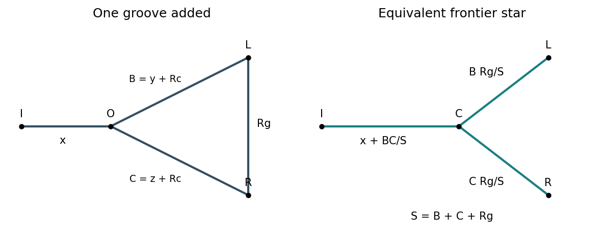
This method retains unequal pressure drops and unequal flow division along the rails; their finite resistances cannot be ignored when assigning the groove flows.
Past exam of the MPhil in micro- and nanotechnology enterprise course of the University of Cambridge 2019 Paper 2 Section A(iii) 19 i Solution by Codex 0 2026-10-20
Codex 0 2026-10-20Negligible rail resistance makes all left-hand groove ends equipotential and all right-hand ends equipotential. The equal hydraulic resistances therefore connect in parallel:Here uses the total inlet flow. The two blind rail ends carry no flow beyond their final grooves.
Past exam of the MPhil in micro- and nanotechnology enterprise course of the University of Cambridge 2019 Paper 2 Section A(iii) 18 iii Solution by Codex 0 2026-10-20
Codex 0 2026-10-20 Past exam of the MPhil in micro- and nanotechnology enterprise course of the University of Cambridge 2019 Paper 2 Section A(iii) 18 i Solution by Codex 0 2026-10-20
Codex 0 2026-10-20 Past exam of the MPhil in micro- and nanotechnology enterprise course of the University of Cambridge 2019 Paper 2 Section A(iii) 17 iv Solution by Codex 0 2026-10-20
Codex 0 2026-10-20 Past exam of the MPhil in micro- and nanotechnology enterprise course of the University of Cambridge 2019 Paper 2 Section A(iii) 17 iii Solution by Codex 0 2026-10-20
Codex 0 2026-10-20 Past exam of the MPhil in micro- and nanotechnology enterprise course of the University of Cambridge 2019 Paper 2 Section A(iii) 17 ii Solution by Codex 0 2026-10-20
Codex 0 2026-10-20 Past exam of the MPhil in micro- and nanotechnology enterprise course of the University of Cambridge 2019 Paper 2 Section A(iii) 17 i Solution by Codex 0 2026-10-20
Codex 0 2026-10-20 Past exam of the MPhil in micro- and nanotechnology enterprise course of the University of Cambridge 2019 Paper 2 Section A(ii) 16 iii Solution by Codex 0 2026-10-20
Codex 0 2026-10-20Spin-valve read-head noise limits the field-to-electrical response: sensitivity is a response relative to noise, not merely a large total resistance. A small free-layer volume gives larger thermally driven angular fluctuations and can lose magnetic stability when its anisotropy barrier is insufficient compared with . Edge damage, stray coupling to the reference layer, nonuniform domains and Barkhausen jumps cause hysteresis and noise. Johnson noise and low-frequency resistance noise compete with a limited GMR signal; raising sense current is restricted by heating and current-induced disturbance.
One useful design combines a single-domain, gently biased free layer with a flux-compensated synthetic-antiferromagnetic reference. This reduces reference stray fields, suppresses unstable domain switching and holds the free layer near a linear operating point. The active sensing width can remain small while magnetic and electrical design preserve adequate stability and signal. An alternative is a magnetic tunnel junction with an optimized barrier, giving a larger magnetoresistance signal; its resistance-area product, shot noise and barrier reliability still require optimization. Shrinking every magnetic dimension indefinitely is not a sensitivity improvement.
[ref]
Giant room-temperature magnetoresistance in Fe-MgO-Fe junctions by Shinji Yuasa and others. Demonstration of large tunnel magnetoresistance with a crystalline MgO barrier
Past exam of the MPhil in micro- and nanotechnology enterprise course of the University of Cambridge 2019 Paper 2 Section A(ii) 16 ii Solution by Codex 0 2026-10-20
Codex 0 2026-10-20For collinear saturated layers, , where . Thus parallel states have and , whereas antiparallel states have and . The free layer switches in the smaller-field interval; the reference layer switches only at larger fields and its loop is shifted by exchange bias.
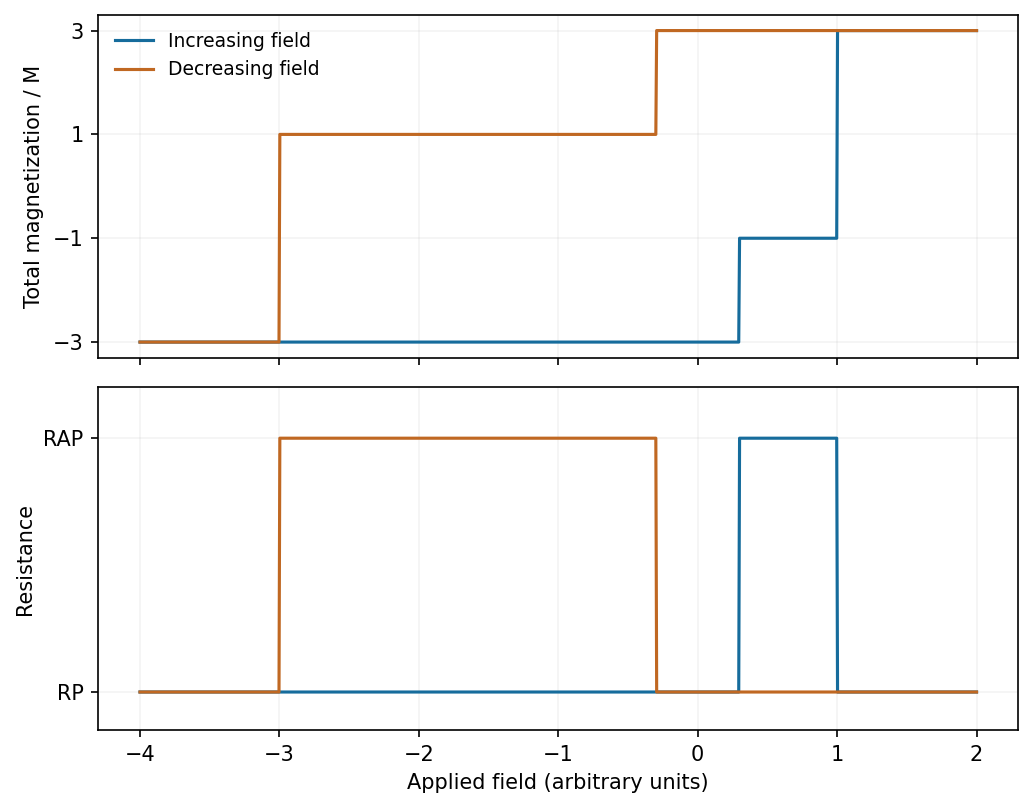
Illustrative major magnetization and resistance loops, with an exchange-shifted reference-layer reversal
. Source. Details. Past exam of the MPhil in micro- and nanotechnology enterprise course of the University of Cambridge 2019 Paper 2 Section A(ii) 16 i Solution by Codex 0 2026-10-20
Codex 0 2026-10-20A spin valve contains a magnetically soft free ferromagnet, a thin nonmagnetic metallic spacer and a reference ferromagnet pinned by exchange bias from an antiferromagnet. The recording track's stray field rotates or reverses the free-layer moment while the reference remains approximately fixed. Spin-dependent scattering makes the resistance lower for parallel moments and higher for antiparallel moments. A sense current converts this into a voltage signal, or a fixed voltage into a current signal.
A useful angular approximation is . Biasing the equilibrium moments near gives an approximately linear response to small track fields. Pinning stability, magnetic shielding and the sensor's spatial extent matter for reading adjacent narrow bits.[ref]
Pinned article: Introduction to the OurBigBook Project
Welcome to the OurBigBook Project! Our goal is to create the perfect publishing platform for STEM subjects, and get university-level students to write the best free STEM tutorials ever.
Everyone is welcome to create an account and play with the site: ourbigbook.com/go/register. We belive that students themselves can write amazing tutorials, but teachers are welcome too. You can write about anything you want, it doesn't have to be STEM or even educational. Silly test content is very welcome and you won't be penalized in any way. Just keep it legal!
Intro to OurBigBook
. Source. We have two killer features:
- topics: topics group articles by different users with the same title, e.g. here is the topic for the "Fundamental Theorem of Calculus" ourbigbook.com/go/topic/fundamental-theorem-of-calculusArticles of different users are sorted by upvote within each article page. This feature is a bit like:
- a Wikipedia where each user can have their own version of each article
- a Q&A website like Stack Overflow, where multiple people can give their views on a given topic, and the best ones are sorted by upvote. Except you don't need to wait for someone to ask first, and any topic goes, no matter how narrow or broad
This feature makes it possible for readers to find better explanations of any topic created by other writers. And it allows writers to create an explanation in a place that readers might actually find it.
Figure 1. Screenshot of the "Derivative" topic page. View it live at: ourbigbook.com/go/topic/derivativeVideo 2. OurBigBook Web topics demo. Source. - local editing: you can store all your personal knowledge base content locally in a plaintext markup format that can be edited locally and published either:This way you can be sure that even if OurBigBook.com were to go down one day (which we have no plans to do as it is quite cheap to host!), your content will still be perfectly readable as a static site.
- to OurBigBook.com to get awesome multi-user features like topics and likes
- as HTML files to a static website, which you can host yourself for free on many external providers like GitHub Pages, and remain in full control

Figure 2. You can publish local OurBigBook lightweight markup files to either OurBigBook.com or as a static website.
Figure 3. Visual Studio Code extension installation.
Figure 5. . You can also edit articles on the Web editor without installing anything locally. Video 3. Edit locally and publish demo. Source. This shows editing OurBigBook Markup and publishing it using the Visual Studio Code extension. 
- Infinitely deep tables of contents:




All our software is open source and hosted at: github.com/ourbigbook/ourbigbook
Further documentation can be found at: docs.ourbigbook.com
Feel free to reach our to us for any help or suggestions: docs.ourbigbook.com/#contact